本周课程主要讲解了如何调参以及batch-norm算法,要点: - 如何调参 - batch norm - 深度学习框架
学习目标:
- Master the process of hyperparameter tuning
课程笔记
Hyperparameter tuning, Batch Normalization and Programming Frameworks
Tuning process
Hyperparameters,常见的超参数:
- learning rate $ $
- 动量超参数 $ $
- 默认值 0.9
- #hidden units
- mini_batch size
- #layers
- learning rate decay
- Adam优化算法 $ _1,_2,$
- 一般取默认值
- $ _1 = 0.9 $
- $ _2 = 0.999 $
- $ = 10^{-8} $
两个原则:
- Try random values: Don't use a grid
- 随机取值,而不是按规律取值
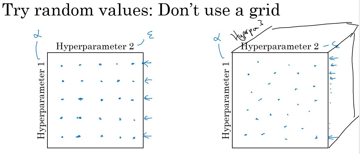
- Coarse to fine: 从粗到细
- 先在大范围内取随机值,然后在表现较好的小区域内取更多的值
Using an appropriate scale to pick hyperparameters
随机抽样并不意味着在有效值范围内的均匀随机抽样(sampleing uniformly at random)。相反,更重要的是选取适当的尺度(scale),用以研究这些超参数。
比如,取\(\alpha\),选定范围\([0.0001,1]\)。 如果直接随机选取,则90%的概率落在\([0.1,1]\)之间,显然是不合理的。 我们需要在\([0.0001,0.001],[0.001,0.01],[0.01,0.1],[0.1,1]\)这4个区间是均匀的。
可以通过取$ r = -4 * np.random.rand()$,r的取值在[-4,0]上随机分布。 然后再取 \(\alpha = 10^r\),取值范围就是\([0.0001,1]\)。
这种是对然尺度,\(10^a - 10^b\)。
再比如$ $,取[0.9,0.999],随机也不太好取。
而$ 1 - $的范围在[0.001,0.1]上,可以转换为上面的方式。
解释:
$ ,0.9000 -> 0.9005$对结果影响非常小。 $ ,0.999 -> 0.9995$对结果影响非常大。
Hyperparameters tuning in practice: Pandas vs. Caviar
原则:
- Baby sitting one model:精心照料某个单一模型。类似 Panda,一胎一个,计算资源稀少
- Training many modes inparallel: 并行训练多个模型。像Caviar,鱼卵,计算资源多
Batch Normalization 批量归一化
Normalizing activations in a network
在深度学习不断兴起的过程中,最重要的创新之一是一种叫批量归一化 (Batch Normalization)的算法,它由Sergey Ioffe 和 Christian Szegedy提出。
- 可以让你的超参搜索变得很简单
- 让你的神经网络变得更加具有鲁棒性
- 可以让你的神经网络对于超参数的选择上不再那么敏感
- 可以让你更容易地训练非常深的网络
Batch norm的实现
Given some internediate values in NN \(z^{(1)},z^{(2)},...,z^{(i)},...,z^{(m)}\)
\[ \mu = \frac{1}{m} \sum_{i=1}^m z^{(i)} \]
\[ \sigma ^ {2} = \frac{1}{m} \sum_{i=1}^m (z^{(i)})^2 \]
\[ z^{(i)}_{norm} = \frac{x - \mu}{\sqrt{\sigma ^2 - \epsilon}} \]
\[ \tilde{z}^{(i)}_{norm} = \gamma z^{(i)}_{norm} + \beta \]
其中 \(\gamma \,\, \beta\)从模型中学习得到。
如果 $= \(,\) = $,则
\[ \tilde{z}^{(i)}_{norm} = z^{(i)}_{norm} \]
也就是说,选择不同的 \(\gamma \,\, \beta\),可以使不同的隐藏层呈现不同的均值和方差的正态分布。
Fitting Batch Norm into a neural network
上面是讲的神经网络的原理。下面讲如何在神经网络中实现batch norm。


Why does Batch Norm work?
为什么BN算法有效? 其中一个理由是,经过归一化的输入特征(用X表示),它们的均值为0、 方差为1,这将大幅加速学习过程,所以与其含有某些在0到1范围内变动的特征、或在1到1000范围内变动的特征,通过归一化所有输入特征X,让它们都拥有相同的变化范围将加速学习。BN算法有效的第二个原因是,它产生权重 (w参数) 在深层次网络中,假设在10层的参数w,比神经网络初始的层级,假设为0层, 更具鲁棒性。
BN算法削弱了前面层参数和后层参数之间的耦合,所以它允许网络的每一层独立学习,有一点独立于其它层的意思,所以这将有效提升整个网络学习速度。但是结论是,BN算法意味着,尤其是从神经网络某一后层角度来看,前面的层的影响并不会很大,因为它们被同一均值和方差所限制,所以这使后层的学习工作变得更加简单。 BN算法还有第二个效果,它具有轻微的正则化效果。
Batch Norm as regularization:
- Each mini-batch is scaled by the mean/variance computed on just that mini-batch.
- This adds some noise to the values 𝑧^([𝑙]) within that minibatch. So similar to dropout, it adds some noise to each hidden layer’s activations.
- This has a slight regularization effect.
Batch Norm at test time

Multi-class classification
Softmax Regression
softmax用于解决多分类的问题。
计算公式为:
\[ z = (\textbf{w}_j^{T}\textbf{x} + b_j) \]
\[ p(y = j|\textbf{z}) = \frac{e^z}{\sum_{j=1}^{m} {e^{z}} } \]
Training a softmax classifier
训练中,使用softmax作为最后一层的输出,最重要的是如何定义损失函数。
和逻辑回归的问题类似,softmax的损失函数定义为:
\[ \begin{aligned} J(\theta) = - \left[ \sum_{i=1}^{m} \sum_{k=1}^{K} 1\left\{y^{(i)} = k\right\} \log \frac{\exp(\theta^{(k)\top} x^{(i)})}{\sum_{j=1}^K \exp(\theta^{(j)\top} x^{(i)})}\right] \end{aligned} \]
Introduction to programming frameworks
Deep learning frameworks
常见的深度网络框架:
- Caffe/Caffe2
- CNTK
- DL4J
- Keras
- Lasagne
- mxnet
- PaddlePaddle
- TensorFlow
- Theano
- Torch
TensorFlow
介绍一些tensorflow的简单示例。
Programming assignment
编程作业: TensorFlow Tutorial
Welcome to this week's programming assignment. Until now, you've always used numpy to build neural networks. Now we will step you through a deep learning framework that will allow you to build neural networks more easily. Machine learning frameworks like TensorFlow, PaddlePaddle, Torch, Caffe, Keras, and many others can speed up your machine learning development significantly. All of these frameworks also have a lot of documentation, which you should feel free to read. In this assignment, you will learn to do the following in TensorFlow:
- Initialize variables
- Start your own session
- Train algorithms
- Implement a Neural Network
Programing frameworks can not only shorten your coding time, but sometimes also perform optimizations that speed up your code.
1 - Exploring the Tensorflow Library
To start, you will import the library:
1 | import math |
Now that you have imported the library, we will walk you through its different applications. You will start with an example, where we compute for you the loss of one training example. \[loss = \mathcal{L}(\hat{y}, y) = (\hat y^{(i)} - y^{(i)})^2 \tag{1}\]
1 |
|
Writing and running programs in TensorFlow has the following steps:
- Create Tensors (variables) that are not yet executed/evaluated.
- Write operations between those Tensors.
- Initialize your Tensors.
- Create a Session.
- Run the Session. This will run the operations you'd written above.
Therefore, when we created a variable for the loss, we simply defined the loss as a function of other quantities, but did not evaluate its value. To evaluate it, we had to run init=tf.global_variables_initializer(). That initialized the loss variable, and in the last line we were finally able to evaluate the value of loss and print its value.
Now let us look at an easy example. Run the cell below:
1 | a = tf.constant(2) |
As expected, you will not see 20! You got a tensor saying that the result is a tensor that does not have the shape attribute, and is of type "int32". All you did was put in the 'computation graph', but you have not run this computation yet. In order to actually multiply the two numbers, you will have to create a session and run it.
1 | sess = tf.Session() |
Great! To summarize, remember to initialize your variables, create a session and run the operations inside the session.
Next, you'll also have to know about placeholders. A placeholder is an object whose value you can specify only later. To specify values for a placeholder, you can pass in values by using a "feed dictionary" (feed_dict variable). Below, we created a placeholder for x. This allows us to pass in a number later when we run the session.
1 | # Change the value of x in the feed_dict |
When you first defined x you did not have to specify a value for it. A placeholder is simply a variable that you will assign data to only later, when running the session. We say that you feed data to these placeholders when running the session.
Here's what's happening: When you specify the operations needed for a computation, you are telling TensorFlow how to construct a computation graph. The computation graph can have some placeholders whose values you will specify only later. Finally, when you run the session, you are telling TensorFlow to execute the computation graph.
1.1 - Linear function
Lets start this programming exercise by computing the following equation: \(Y = WX + b\), where \(W\) and \(X\) are random matrices and b is a random vector.
Exercise: Compute \(WX + b\) where \(W, X\), and \(b\) are drawn from a random normal distribution. W is of shape (4, 3), X is (3,1) and b is (4,1). As an example, here is how you would define a constant X that has shape (3,1): 1
2X = tf.constant(np.random.randn(3,1), name = "X")
1 | # GRADED FUNCTION: linear_function |
1.2 - Computing the sigmoid
Great! You just implemented a linear function. Tensorflow offers a variety of commonly used neural network functions like tf.sigmoid and tf.softmax. For this exercise lets compute the sigmoid function of an input.
You will do this exercise using a placeholder variable x. When running the session, you should use the feed dictionary to pass in the input z. In this exercise, you will have to (i) create a placeholder x, (ii) define the operations needed to compute the sigmoid using tf.sigmoid, and then (iii) run the session.
** Exercise **: Implement the sigmoid function below. You should use the following:
tf.placeholder(tf.float32, name = "...")tf.sigmoid(...)sess.run(..., feed_dict = {x: z})
Note that there are two typical ways to create and use sessions in tensorflow:
Method 1: 1
2
3
4sess = tf.Session()
# Run the variables initialization (if needed), run the operations
result = sess.run(..., feed_dict = {...})
sess.close() # Close the session1
2
3
4with tf.Session() as sess:
# run the variables initialization (if needed), run the operations
result = sess.run(..., feed_dict = {...})
# This takes care of closing the session for you :)
1 | # GRADED FUNCTION: sigmoid |
To summarize, you how know how to: 1. Create placeholders 2. Specify the computation graph corresponding to operations you want to compute 3. Create the session 4. Run the session, using a feed dictionary if necessary to specify placeholder variables' values.
1.3 - Computing the Cost
You can also use a built-in function to compute the cost of your neural network. So instead of needing to write code to compute this as a function of \(a^{[2](i)}\) and \(y^{(i)}\) for i=1...m: \[ J = - \frac{1}{m} \sum_{i = 1}^m \large ( \small y^{(i)} \log a^{ [2] (i)} + (1-y^{(i)})\log (1-a^{ [2] (i)} )\large )\small\]
you can do it in one line of code in tensorflow!
Exercise: Implement the cross entropy loss. The function you will use is:
tf.nn.sigmoid_cross_entropy_with_logits(logits = ..., labels = ...)
Your code should input z, compute the sigmoid (to get a) and then compute the cross entropy cost \(J\). All this can be done using one call to tf.nn.sigmoid_cross_entropy_with_logits, which computes
\[- \frac{1}{m} \sum_{i = 1}^m \large ( \small y^{(i)} \log \sigma(z^{[2](i)}) + (1-y^{(i)})\log (1-\sigma(z^{[2](i)})\large )\small\]
1 | # GRADED FUNCTION: cost |
1.4 - Using One Hot encodings
Many times in deep learning you will have a y vector with numbers ranging from 0 to C-1, where C is the number of classes. If C is for example 4, then you might have the following y vector which you will need to convert as follows:
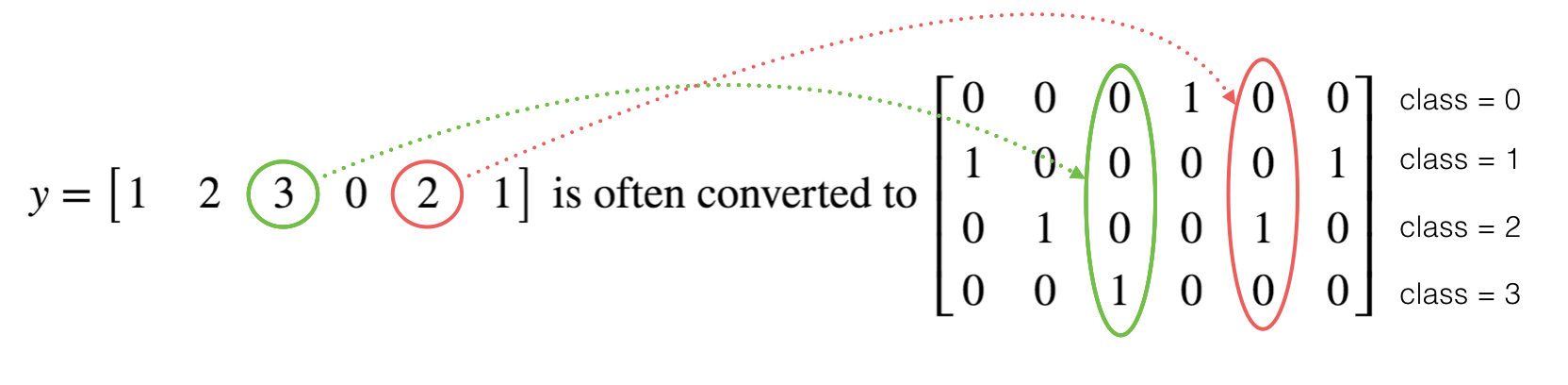
This is called a "one hot" encoding, because in the converted representation exactly one element of each column is "hot" (meaning set to 1). To do this conversion in numpy, you might have to write a few lines of code. In tensorflow, you can use one line of code:
- tf.one_hot(labels, depth, axis)
Exercise: Implement the function below to take one vector of labels and the total number of classes \(C\), and return the one hot encoding. Use tf.one_hot() to do this.
1 | # GRADED FUNCTION: one_hot_matrix |
1.5 - Initialize with zeros and ones
Now you will learn how to initialize a vector of zeros and ones. The function you will be calling is tf.ones(). To initialize with zeros you could use tf.zeros() instead. These functions take in a shape and return an array of dimension shape full of zeros and ones respectively.
Exercise: Implement the function below to take in a shape and to return an array (of the shape's dimension of ones).
- tf.ones(shape)
1 | # GRADED FUNCTION: ones |
2 - Building your first neural network in tensorflow
In this part of the assignment you will build a neural network using tensorflow. Remember that there are two parts to implement a tensorflow model:
- Create the computation graph
- Run the graph
Let's delve into the problem you'd like to solve!
2.0 - Problem statement: SIGNS Dataset
One afternoon, with some friends we decided to teach our computers to decipher sign language. We spent a few hours taking pictures in front of a white wall and came up with the following dataset. It's now your job to build an algorithm that would facilitate communications from a speech-impaired person to someone who doesn't understand sign language.
- Training set: 1080 pictures (64 by 64 pixels) of signs representing numbers from 0 to 5 (180 pictures per number).
- Test set: 120 pictures (64 by 64 pixels) of signs representing numbers from 0 to 5 (20 pictures per number).
Note that this is a subset of the SIGNS dataset. The complete dataset contains many more signs.
Here are examples for each number, and how an explanation of how we represent the labels. These are the original pictures, before we lowered the image resolutoion to 64 by 64 pixels.

Run the following code to load the dataset.
1 | #Loading the dataset |
Change the index below and run the cell to visualize some examples in the dataset.
1 | # Example of a picture |
As usual you flatten the image dataset, then normalize it by dividing by 255. On top of that, you will convert each label to a one-hot vector as shown in Figure 1. Run the cell below to do so.
1 | #Flatten the training and test images |
Output 1
2
3
4
5
6number of training examples = 1080
number of test examples = 120
X_train shape: (12288, 1080)
Y_train shape: (6, 1080)
X_test shape: (12288, 120)
Y_test shape: (6, 120)
Note that 12288 comes from \(64 \times 64 \times 3\). Each image is square, 64 by 64 pixels, and 3 is for the RGB colors. Please make sure all these shapes make sense to you before continuing.
Your goal is to build an algorithm capable of recognizing a sign with high accuracy. To do so, you are going to build a tensorflow model that is almost the same as one you have previously built in numpy for cat recognition (but now using a softmax output). It is a great occasion to compare your numpy implementation to the tensorflow one.
The model is LINEAR -> RELU -> LINEAR -> RELU -> LINEAR -> SOFTMAX. The SIGMOID output layer has been converted to a SOFTMAX. A SOFTMAX layer generalizes SIGMOID to when there are more than two classes.
2.1 - Create placeholders
Your first task is to create placeholders for X and Y. This will allow you to later pass your training data in when you run your session.
Exercise: Implement the function below to create the placeholders in tensorflow.
1 | # GRADED FUNCTION: create_placeholders |
2.2 - Initializing the parameters
Your second task is to initialize the parameters in tensorflow.
Exercise: Implement the function below to initialize the parameters in tensorflow. You are going use Xavier Initialization for weights and Zero Initialization for biases. The shapes are given below. As an example, to help you, for W1 and b1 you could use:
1 | W1 = tf.get_variable("W1", [25,12288], initializer = tf.contrib.layers.xavier_initializer(seed = 1)) |
Please use seed = 1 to make sure your results match ours.
1 | # GRADED FUNCTION: initialize_parameters |
As expected, the parameters haven't been evaluated yet.
2.3 - Forward propagation in tensorflow
You will now implement the forward propagation module in tensorflow. The function will take in a dictionary of parameters and it will complete the forward pass. The functions you will be using are:
tf.add(...,...)to do an additiontf.matmul(...,...)to do a matrix multiplicationtf.nn.relu(...)to apply the ReLU activation
Question: Implement the forward pass of the neural network. We commented for you the numpy equivalents so that you can compare the tensorflow implementation to numpy. It is important to note that the forward propagation stops at z3. The reason is that in tensorflow the last linear layer output is given as input to the function computing the loss. Therefore, you don't need a3!
1 | #GRADED FUNCTION: forward_propagation |
You may have noticed that the forward propagation doesn't output any cache. You will understand why below, when we get to brackpropagation.
2.4 Compute cost
As seen before, it is very easy to compute the cost using: 1
tf.reduce_mean(tf.nn.softmax_cross_entropy_with_logits(logits = ..., labels = ...))
logits" and "labels" inputs of tf.nn.softmax_cross_entropy_with_logits are expected to be of shape (number of examples, num_classes). We have thus transposed Z3 and Y for you. - Besides, tf.reduce_mean basically does the summation over the examples.
1 | #GRADED FUNCTION: compute_cost |
2.5 - Backward propagation & parameter updates
This is where you become grateful to programming frameworks. All the backpropagation and the parameters update is taken care of in 1 line of code. It is very easy to incorporate this line in the model.
After you compute the cost function. You will create an "optimizer" object. You have to call this object along with the cost when running the tf.session. When called, it will perform an optimization on the given cost with the chosen method and learning rate.
For instance, for gradient descent the optimizer would be: 1
optimizer = tf.train.GradientDescentOptimizer(learning_rate = learning_rate).minimize(cost)
To make the optimization you would do: 1
_ , c = sess.run([optimizer, cost], feed_dict={X: minibatch_X, Y: minibatch_Y})
This computes the backpropagation by passing through the tensorflow graph in the reverse order. From cost to inputs.
Note When coding, we often use _ as a "throwaway" variable to store values that we won't need to use later. Here, _ takes on the evaluated value of optimizer, which we don't need (and c takes the value of the cost variable).
2.6 - Building the model
Now, you will bring it all together!
Exercise: Implement the model. You will be calling the functions you had previously implemented.
1 |
|
Run the following cell to train your model! On our machine it takes about 5 minutes. Your "Cost after epoch 100" should be 1.016458. If it's not, don't waste time; interrupt the training by clicking on the square (⬛) in the upper bar of the notebook, and try to correct your code. If it is the correct cost, take a break and come back in 5 minutes!
Amazing, your algorithm can recognize a sign representing a figure between 0 and 5 with 71.7% accuracy.
Insights: - Your model seems big enough to fit the training set well. However, given the difference between train and test accuracy, you could try to add L2 or dropout regularization to reduce overfitting. - Think about the session as a block of code to train the model. Each time you run the session on a minibatch, it trains the parameters. In total you have run the session a large number of times (1500 epochs) until you obtained well trained parameters.
2.7 - Test with your own image (optional / ungraded exercise)
Congratulations on finishing this assignment. You can now take a picture of your hand and see the output of your model. To do that: 1. Click on "File" in the upper bar of this notebook, then click "Open" to go on your Coursera Hub. 2. Add your image to this Jupyter Notebook's directory, in the "images" folder 3. Write your image's name in the following code 4. Run the code and check if the algorithm is right!
1 | import scipy |
You indeed deserved a "thumbs-up" although as you can see the algorithm seems to classify it incorrectly. The reason is that the training set doesn't contain any "thumbs-up", so the model doesn't know how to deal with it! We call that a "mismatched data distribution" and it is one of the various of the next course on "Structuring Machine Learning Projects".
What you should remember:
- Tensorflow is a programming framework used in deep learning
- The two main object classes in tensorflow are Tensors and Operators.
- When you code in tensorflow you have to take the following steps:
- Create a graph containing Tensors (Variables, Placeholders ...) and Operations (tf.matmul, tf.add, ...)
- Create a session
- Initialize the session
- Run the session to execute the graph
- You can execute the graph multiple times as you've seen in model()
- The backpropagation and optimization is automatically done when running the session on the "optimizer" object.