本周课程主要讲解了神经网络的一些优化算法,要点: - 随机梯度下降 - Momentum(动量)优化算法 - RMSProp优化算法 - Adam优化算法
学习目标 - Remember different optimization methods such as (Stochastic) Gradient Descent, Momentum, RMSProp and Adam - Use random minibatches to accelerate the convergence and improve the optimization - Know the benefits of learning rate decay and apply it to your optimization
课程笔记
Optimization algorithms
Mini-batch gradient descent
Mini-batch gradient descent(小批量梯度下降法)
如果训练集非常大,比如m = 5,000,000 ,则训练会非常慢。
将训练集拆分成更小的,微小的训练集,即小批量训练集(mini-batch)。比如说每一个微型训练集只有1000个训练样例。如果总共有5百万个训练样例,每个小批量样例有1000个样例,则有5000个这样的小批量样例。

这是小批量梯度下降算法处理训练集一轮的过程,也叫做训练集的一次遍历(epoch)。遍历是指过一遍训练集,只不过在批量梯度下降法中,对训练集的一轮处理只能得到一步逼近,而小批量梯度下降法中对训练集的一轮处理,也就是一次遍历,可以得到5000步梯度逼近。当有一个大型训练集时,小批量梯度下降法比梯度下降法要快得多。
Understanding mini-batch gradient descent

对梯度下降算法,损失函数是随着迭代次数单调递减的。如果某一次迭代它的值增加了那么一定是哪里错了,也许是学习率太大。
而在小批量梯度下降中,同样画图就会发现,并不是每一次迭代代价函数的值都会变小。它的趋势是向下的,但是也会有许多噪声。 如果使用小批量梯度下降算法,经过几轮训练后,对 $ J^{t} \(作图,它并不一定每次迭代都会下降,但是整体趋势必须是向下的,而它之所以有噪声,可能和计算代价函数时使用的那个批次\) X ^ {t}, Y ^ {t}$有关。
mini_batch大小
batch_size = 1 : 随机梯度下降(SDG,stochasit gradient descent) batch_size = m : 批量梯度下降Batch gradient descent
批量梯度下降最大的缺点是,如果训练集非常大,就将在每一次迭代上花费太长的时间。如果你的训练集比较小,它还是一个不错的选择。
随机梯度下降有一个很大的缺点是:失去了可以利用向量加速运算的机会。
如何选Batch_size:
- 1.训练集小( <= 2000): Batch gradient descent
- 2.typical batch_size: 64-512之间的2^n
确保mini-batch 所有的\(X^{t} Y^{t}\) 是可以放进CPU/GPU 内存的 。
Batch Gradient Descent
1 | X = daty_input |
Stochastic Gradient Descent:
1 | X = daty_input |
Mini Batch Gradient descent 准备数据的两个步骤;
- 1.Shuffle:洗牌:把原输入随机打乱,当然要保持X和Y对应一致
- 2.Partition: 分区:按batch_size分区,前面t-1个分区的大小都是batch_size,最后一个可能不足batch_size
Exponentially weighted averages
指数加权平均

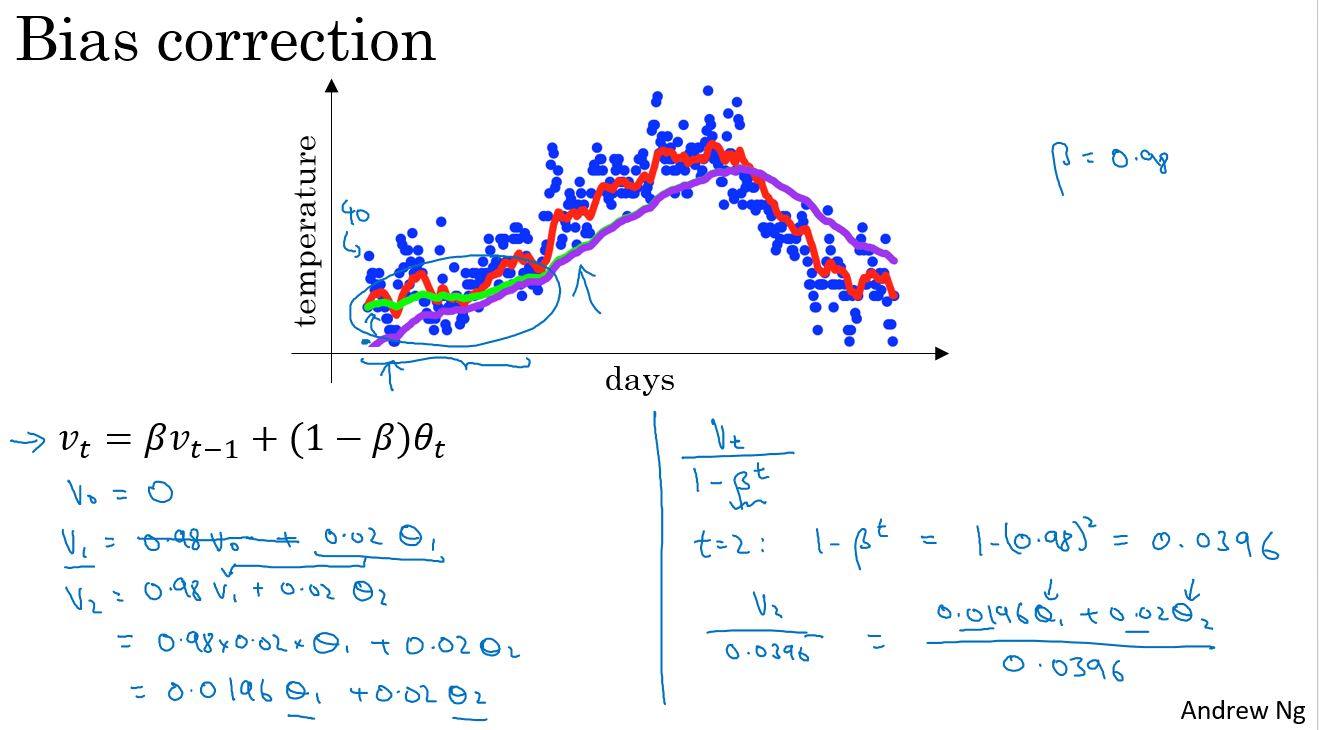
红线表示\(\theta\) = 0.9 绿线表示\(\theta\) = 0.98 黄线表示\(\theta\) = 0.5
Understanding exponentially weighted averages

Bias correction in exponentially weighted averages
这里有一个技术细节,称为偏差修正,它能帮助更精确地计算平均值。
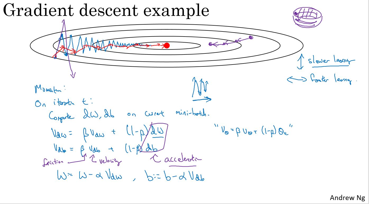
Gradient descent with momentum
有一种算法叫做动量(Momentum)或者叫动量梯度下降算法,它几乎总会比标准的梯度下降算法更快。一言以蔽之,算法的主要思想是:计算梯度的指数加权平均,然后使用这个梯度来更新权重。

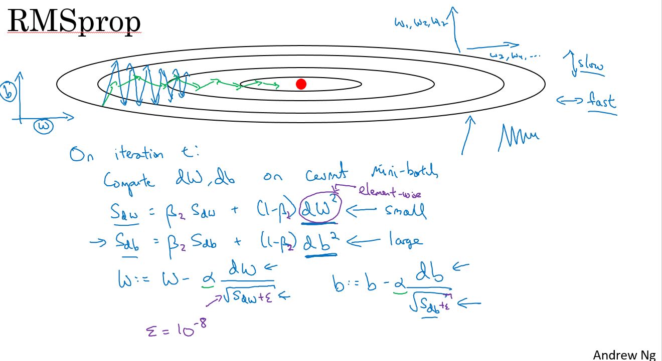
RMSprop
上面已经学习了如何用动量来加速梯度下降,还有一个叫做RMSprop的算法,全称为均方根传递(Root Mean Square prop)。它也可以加速梯度下降。我们来看看它是如何工作的。
之前的例子中,在实现梯度下降时,可能会在垂直方向上出现巨大的振荡,即使它试图在水平方向上前进。为了说明这个例子,假设,纵轴代表参数b,横轴代表参数W,当然这里也可以是W1和W2等其他参数。使用b和W是为了便于理解,我们希望减慢b方向的学习,也就是垂直方向,同时加速或至少不减慢水平方向的学习,这就是RMSprop算法要做的。
Adam optimization algorithm
有些人尝试把梯度下降与动量算法结合起来,结果非常有效。而至今也并没有出现效果比它好很多的优化算法。关于RMSProp和Adam优化算法,属于其中极少数真正有效的算法,适用于很多不同的深度学习网络结构。
Adam优化算法本质上是将动量算法和RMSprop结合起来。

Learning rate decay
有一种方法或许能学习算法运行更快,那就是渐渐地减小学习率,称之为学习率衰减。

The problem of local optima
在深度学习的早期阶段,人们常常担心优化算法,会陷入糟糕的局部最优(Local Optima)之中,但随着深度学习理论的发展,对局部最优的理解也在改变。

假设在一个2万维的空间中,如果一个点要成为局部最优,则需要在所有的2万个方向上都凹或者凸,因此这件事发生的概率非常低,大概2的负2万次方。更有可能遇到的情况是,某些方向的曲线像这样向上弯曲,同时另一些方向的曲线则向下弯曲,并非所有曲线都向上弯曲,这就是为什么在高维空间中,更有可能碰到一个像上图这样的鞍点,而不是局部最优。
更有可能遇到鞍点,而不是局部最优。如果局部最优不是问题,问题是会降低学习速度。实际上是停滞区(Plateaus)。停滞区指的是,导数长时间接近于零的一段区域。如果你在这里,那么梯度下降会沿着这个曲面向下移动,然而因为梯度为零或接近于零,曲面很平,会花费很长的时间,缓慢地在停滞区里找到这个点,然后因为左侧或右侧的随机扰动。算法终于能够离开这个停滞区,它一直沿着这个很长的坡往下走,离开这个停滞区。
像动量(Momentum)算法或RmsProp算法或Adam算法能改善学习算法的地方,就是在这些场景下,可以加快沿停滞区向下移动。然后离开停滞区的速度。
Programming assignment
编程作业: Optimization
Optimization Methods
Until now, you've always used Gradient Descent to update the parameters and minimize the cost. In this notebook, you will learn more advanced optimization methods that can speed up learning and perhaps even get you to a better final value for the cost function. Having a good optimization algorithm can be the difference between waiting days vs. just a few hours to get a good result.
Gradient descent goes "downhill" on a cost function \(J\). Think of it as trying to do this:

Notations: As usual, $ = $ da for any variable a.
To get started, run the following code to import the libraries you will need.
1 | import numpy as np |
1 | get_ipython().magic('matplotlib inline') |
1 - Gradient Descent
A simple optimization method in machine learning is gradient descent (GD). When you take gradient steps with respect to all \(m\) examples on each step, it is also called Batch Gradient Descent.
Warm-up exercise: Implement the gradient descent update rule. The gradient descent rule is, for \(l = 1, ..., L\): \[ W^{[l]} = W^{[l]} - \alpha \text{ } dW^{[l]} \]
\[ b^{[l]} = b^{[l]} - \alpha \text{ } db^{[l]} \]
where L is the number of layers and \(\alpha\) is the learning rate. All parameters should be stored in the parameters dictionary. Note that the iterator l starts at 0 in the for loop while the first parameters are \(W^{[1]}\) and \(b^{[1]}\). You need to shift l to l+1 when coding.
1 | # GRADED FUNCTION: update_parameters_with_gd |
A variant of this is Stochastic Gradient Descent (SGD), which is equivalent to mini-batch gradient descent where each mini-batch has just 1 example. The update rule that you have just implemented does not change. What changes is that you would be computing gradients on just one training example at a time, rather than on the whole training set. The code examples below illustrate the difference between stochastic gradient descent and (batch) gradient descent.
- (Batch) Gradient Descent:
1 | X = data_input |
- Stochastic Gradient Descent:
1 | X = data_input |
In Stochastic Gradient Descent, you use only 1 training example before updating the gradients. When the training set is large, SGD can be faster. But the parameters will "oscillate" toward the minimum rather than converge smoothly. Here is an illustration of this:
.")
Figure 1: SGD vs GD, denotes a minimum of the cost. SGD leads to many oscillations to reach convergence. But each step is a lot faster to compute for SGD than for GD, as it uses only one training example (vs. the whole batch for GD).
Note also that implementing SGD requires 3 for-loops in total: 1. Over the number of iterations 2. Over the \(m\) training examples 3. Over the layers (to update all parameters, from \((W^{[1]},b^{[1]})\) to \((W^{[L]},b^{[L]})\))
In practice, you'll often get faster results if you do not use neither the whole training set, nor only one training example, to perform each update. Mini-batch gradient descent uses an intermediate number of examples for each step. With mini-batch gradient descent, you loop over the mini-batches instead of looping over individual training examples.

What you should remember: - The difference between gradient descent, mini-batch gradient descent and stochastic gradient descent is the number of examples you use to perform one update step. - You have to tune a learning rate hyperparameter \(\alpha\). - With a well-turned mini-batch size, usually it outperforms either gradient descent or stochastic gradient descent (particularly when the training set is large).
2 - Mini-Batch Gradient descent
Let's learn how to build mini-batches from the training set (X, Y).
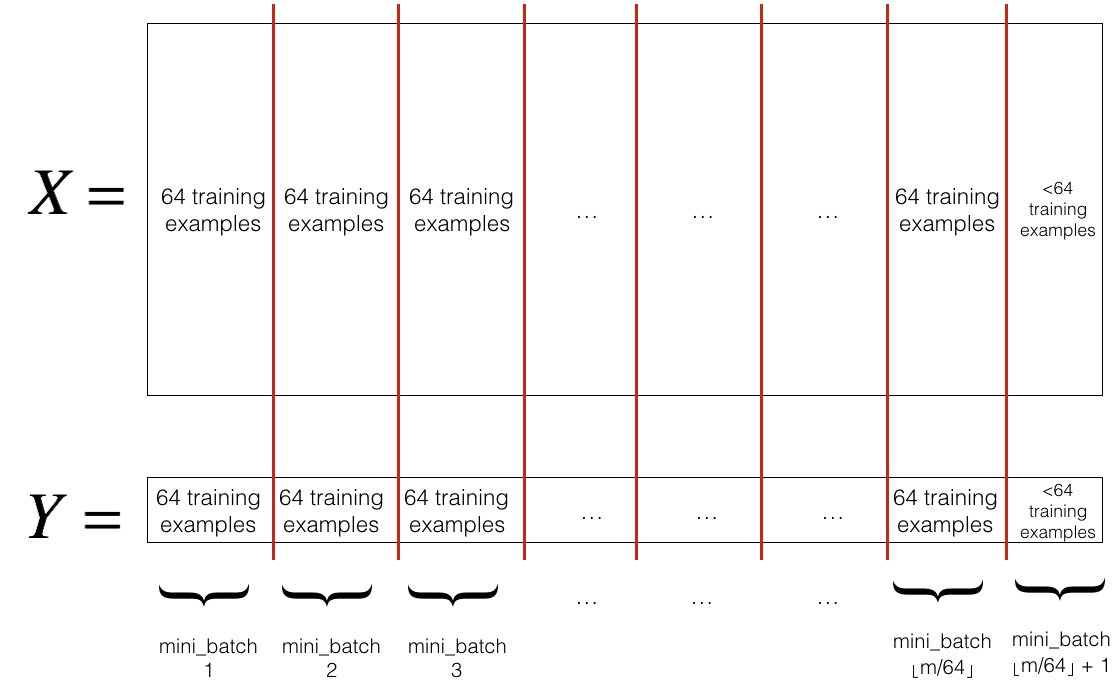
There are two steps: - Shuffle: Create a shuffled version of the training set (X, Y) as shown below. Each column of X and Y represents a training example. Note that the random shuffling is done synchronously between X and Y. Such that after the shuffling the \(i^{th}\) column of X is the example corresponding to the \(i^{th}\) label in Y. The shuffling step ensures that examples will be split randomly into different mini-batches.
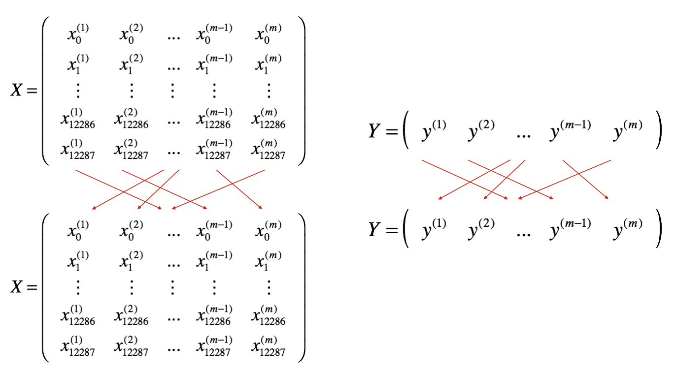
- Partition: Partition the shuffled (X, Y) into mini-batches of size
mini_batch_size(here 64). Note that the number of training examples is not always divisible bymini_batch_size. The last mini batch might be smaller, but you don't need to worry about this. When the final mini-batch is smaller than the fullmini_batch_size, it will look like this:
Exercise: Implement random_mini_batches. We coded the shuffling part for you. To help you with the partitioning step, we give you the following code that selects the indexes for the \(1^{st}\) and \(2^{nd}\) mini-batches: 1
2
3first_mini_batch_X = shuffled_X[:, 0 : mini_batch_size]
second_mini_batch_X = shuffled_X[:, mini_batch_size : 2 * mini_batch_size]
...
Note that the last mini-batch might end up smaller than mini_batch_size=64. Let \(\lfloor s \rfloor\) represents \(s\) rounded down to the nearest integer (this is math.floor(s) in Python). If the total number of examples is not a multiple of mini_batch_size=64 then there will be \(\lfloor \frac{m}{mini\_batch\_size}\rfloor\) mini-batches with a full 64 examples, and the number of examples in the final mini-batch will be (\(m-mini_\_batch_\_size \times \lfloor \frac{m}{mini\_batch\_size}\rfloor\)).
1 | # GRADED FUNCTION: random_mini_batches |
1 | X_assess, Y_assess, mini_batch_size = random_mini_batches_test_case() |
Expected Output:
| shape of the 1st mini_batch_X |
What you should remember: - Shuffling and Partitioning are the two steps required to build mini-batches - Powers of two are often chosen to be the mini-batch size, e.g., 16, 32, 64, 128.
3 - Momentum
Because mini-batch gradient descent makes a parameter update after seeing just a subset of examples, the direction of the update has some variance, and so the path taken by mini-batch gradient descent will "oscillate" toward convergence. Using momentum can reduce these oscillations.
Momentum takes into account the past gradients to smooth out the update. We will store the 'direction' of the previous gradients in the variable \(v\). Formally, this will be the exponentially weighted average of the gradient on previous steps. You can also think of \(v\) as the "velocity" of a ball rolling downhill, building up speed (and momentum) according to the direction of the gradient/slope of the hill.
Exercise: Initialize the velocity. The velocity, \(v\), is a python dictionary that needs to be initialized with arrays of zeros. Its keys are the same as those in the grads dictionary, that is: for \(l =1,...,L\): 1
2v["dW" + str(l+1)] = ... #(numpy array of zeros with the same shape as parameters["W" + str(l+1)])
v["db" + str(l+1)] = ... #(numpy array of zeros with the same shape as parameters["b" + str(l+1)])for loop.
1 | # GRADED FUNCTION: initialize_velocity |
Exercise: Now, implement the parameters update with momentum. The momentum update rule is, for \(l = 1, ..., L\):
\[ \begin{cases} v_{dW^{[l]}} = \beta v_{dW^{[l]}} + (1 - \beta) dW^{[l]} \\ W^{[l]} = W^{[l]} - \alpha v_{dW^{[l]}} \end{cases}\]
\[\begin{cases} v_{db^{[l]}} = \beta v_{db^{[l]}} + (1 - \beta) db^{[l]} \\ b^{[l]} = b^{[l]} - \alpha v_{db^{[l]}} \end{cases}\]
where L is the number of layers, \(\beta\) is the momentum and \(\alpha\) is the learning rate. All parameters should be stored in the parameters dictionary. Note that the iterator l starts at 0 in the for loop while the first parameters are \(W^{[1]}\) and \(b^{[1]}\) (that's a "one" on the superscript). So you will need to shift l to l+1 when coding.
1 | # GRADED FUNCTION: update_parameters_with_momentum |
Note that: - The velocity is initialized with zeros. So the algorithm will take a few iterations to "build up" velocity and start to take bigger steps. - If \(\beta = 0\), then this just becomes standard gradient descent without momentum.
How do you choose \(\beta\)?
- The larger the momentum \(\beta\) is, the smoother the update because the more we take the past gradients into account. But if \(\beta\) is too big, it could also smooth out the updates too much.
- Common values for \(\beta\) range from 0.8 to 0.999. If you don't feel inclined to tune this, \(\beta = 0.9\) is often a reasonable default.
- Tuning the optimal \(\beta\) for your model might need trying several values to see what works best in term of reducing the value of the cost function \(J\).
What you should remember: - Momentum takes past gradients into account to smooth out the steps of gradient descent. It can be applied with batch gradient descent, mini-batch gradient descent or stochastic gradient descent. - You have to tune a momentum hyperparameter \(\beta\) and a learning rate \(\alpha\).
4 - Adam
Adam is one of the most effective optimization algorithms for training neural networks. It combines ideas from RMSProp (described in lecture) and Momentum.
How does Adam work? 1. It calculates an exponentially weighted average of past gradients, and stores it in variables \(v\) (before bias correction) and \(v^{corrected}\) (with bias correction). 2. It calculates an exponentially weighted average of the squares of the past gradients, and stores it in variables \(s\) (before bias correction) and \(s^{corrected}\) (with bias correction). 3. It updates parameters in a direction based on combining information from "1" and "2".
The update rule is, for \(l = 1, ..., L\):
\[\begin{cases} v_{dW^{[l]}} = \beta_1 v_{dW^{[l]}} + (1 - \beta_1) \frac{\partial \mathcal{J} }{ \partial W^{[l]} } \\ v^{corrected}_{dW^{[l]}} = \frac{v_{dW^{[l]}}}{1 - (\beta_1)^t} \\ s_{dW^{[l]}} = \beta_2 s_{dW^{[l]}} + (1 - \beta_2) (\frac{\partial \mathcal{J} }{\partial W^{[l]} })^2 \\ s^{corrected}_{dW^{[l]}} = \frac{s_{dW^{[l]}}}{1 - (\beta_1)^t} \\ W^{[l]} = W^{[l]} - \alpha \frac{v^{corrected}_{dW^{[l]}}}{\sqrt{s^{corrected}_{dW^{[l]}}} + \varepsilon} \end{cases}\] where: - t counts the number of steps taken of Adam - L is the number of layers - \(\beta_1\) and \(\beta_2\) are hyperparameters that control the two exponentially weighted averages. - \(\alpha\) is the learning rate - \(\varepsilon\) is a very small number to avoid dividing by zero
As usual, we will store all parameters in the parameters dictionary
Exercise: Initialize the Adam variables \(v, s\) which keep track of the past information.
Instruction: The variables \(v, s\) are python dictionaries that need to be initialized with arrays of zeros. Their keys are the same as for grads, that is: for \(l = 1, ..., L\): 1
2
3
4
5v["dW" + str(l+1)] = ... #(numpy array of zeros with the same shape as parameters["W" + str(l+1)])
v["db" + str(l+1)] = ... #(numpy array of zeros with the same shape as parameters["b" + str(l+1)])
s["dW" + str(l+1)] = ... #(numpy array of zeros with the same shape as parameters["W" + str(l+1)])
s["db" + str(l+1)] = ... #(numpy array of zeros with the same shape as parameters["b" + str(l+1)])
1 | # GRADED FUNCTION: initialize_adam |
Exercise: Now, implement the parameters update with Adam. Recall the general update rule is, for \(l = 1, ..., L\):
\[\begin{cases} v_{W^{[l]}} = \beta_1 v_{W^{[l]}} + (1 - \beta_1) \frac{\partial J }{ \partial W^{[l]} } \\ v^{corrected}_{W^{[l]}} = \frac{v_{W^{[l]}}}{1 - (\beta_1)^t} \\ s_{W^{[l]}} = \beta_2 s_{W^{[l]}} + (1 - \beta_2) (\frac{\partial J }{\partial W^{[l]} })^2 \\ s^{corrected}_{W^{[l]}} = \frac{s_{W^{[l]}}}{1 - (\beta_2)^t} \\ W^{[l]} = W^{[l]} - \alpha \frac{v^{corrected}_{W^{[l]}}}{\sqrt{s^{corrected}_{W^{[l]}}}+\varepsilon} \end{cases}\]
Note that the iterator l starts at 0 in the for loop while the first parameters are \(W^{[1]}\) and \(b^{[1]}\). You need to shift l to l+1 when coding.
1 | # GRADED FUNCTION: update_parameters_with_adam |
You now have three working optimization algorithms (mini-batch gradient descent, Momentum, Adam). Let's implement a model with each of these optimizers and observe the difference.
5 - Model with different optimization algorithms
Lets use the following "moons" dataset to test the different optimization methods. (The dataset is named "moons" because the data from each of the two classes looks a bit like a crescent-shaped moon.)
1 | train_X, train_Y = load_dataset() |
We have already implemented a 3-layer neural network. You will train it with: - Mini-batch Gradient Descent: it will call your function: - update_parameters_with_gd() - Mini-batch Momentum: it will call your functions: - initialize_velocity() and update_parameters_with_momentum() - Mini-batch Adam: it will call your functions: - initialize_adam() and update_parameters_with_adam()
1 | def model(X, Y, layers_dims, optimizer, learning_rate = 0.0007, mini_batch_size = 64, beta = 0.9, |
You will now run this 3 layer neural network with each of the 3 optimization methods.
5.1 - Mini-batch Gradient descent
Run the following code to see how the model does with mini-batch gradient descent.
1 | train 3-layer model |
5.2 - Mini-batch gradient descent with momentum
Run the following code to see how the model does with momentum. Because this example is relatively simple, the gains from using momemtum are small; but for more complex problems you might see bigger gains.
1 | train 3-layer model |
5.3 - Mini-batch with Adam mode
Run the following code to see how the model does with Adam.
1 | train 3-layer model |
5.4 - Summary
| optimization method | accuracy | cost shape | Gradient descent | 79.7% | oscillations |
| Momentum | 79.7% | oscillations |
| Adam | 94% | smoother |
Momentum usually helps, but given the small learning rate and the simplistic dataset, its impact is almost negligeable. Also, the huge oscillations you see in the cost come from the fact that some minibatches are more difficult thans others for the optimization algorithm.
Adam on the other hand, clearly outperforms mini-batch gradient descent and Momentum. If you run the model for more epochs on this simple dataset, all three methods will lead to very good results. However, you've seen that Adam converges a lot faster.
Some advantages of Adam include: - Relatively low memory requirements (though higher than gradient descent and gradient descent with momentum) - Usually works well even with little tuning of hyperparameters (except \(\alpha\))
References:
- Adam paper: https://arxiv.org/pdf/1412.6980.pdf