课程笔记
本周课程主要讲了卷积神经网络在其他领域的应用,要点: - 艺术风格转换 - 人脸识别
学习目标:
- Discover how CNNs can be applied to multiple fields, including art generation and face recognition. Implement your own algorithm to generate art and recognize faces!
Face Recognition
What is face recognition?
人脸设别和人脸验证的区别:
- 人脸验证
- 输入一副图片,包含名字或ID
- 输出输入普通是否是要确认的人
- 人脸识别
- 一个数据库,包含K个人
- 有个输入图片
- 如果图片是数据库中任何K个人之一,输出这个人的ID,否则输出无法识别

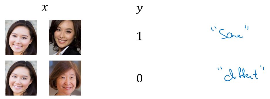
One Shot Learning
One shot Learning问题是指,仅仅从一个实例再次识别这个人。
Learning from one example to recognize the person again。
通过相似度函数来解决此问题。相似度函数定义为:
$ d(img1,img2) = degree, of ,difference, between ,images$
这个函数是用来描述两幅图片的相似度。
1 | If d(img1,img2) ≤ 𝜏 , same person |
Siamese Network(孪生网络)
上一节中学到,函数d的任务是接受两张脸的输入,并输出它们有多相似,或有多不同。 实现这个的一个好办法是Siamese网络。
把输入人脸图片经过一个卷积神经网络推理后,得到了一个特征向量(softmax的前一层)。有时候把它输入到一个softmax层中,去做分类。 这儿不这样做,而是专注在这个向量本身,比如说128个数,它由神经网络深处的某个全连接层计算而来。
给这128个数(组成的向量)起个名字,把它叫做 \(f(x^{(1)})\) 大家可以把f(x1)看成是输入图片x1的编码。同样将第二张图片输入到同一个网络,使用相同的参数,得到一个不同的,128个数字组成的向量,这是第二张图片的编码。 称之为第二张图片的编码,即\(f(x^{(2)}\)。最后,定义距离d是x1和 x2这两张图片的编码之间差的范数。
这种方法,用两个完全相同的卷积神经网络对两张不同的图片进行计算,比较二者的结果,有时称之为孪生网络(Siamese Network)架构。

该如何训练Siamese Network?
训练一个神经网络,使得它计算的编码可以生成一个函数d来判断这两张照片是同一个人的。更正式的来说,神经网络的参数定义了编码f(xi),当给定输入图片xi, 这个神经网络输出这个128维的编码 f(xi)。如果两张图片xi和xj上是同一个人,那么他们的编码的差距就会小。相反的,如果xi和xj上是不同的人,那么你就想要他们的编码的差距大。 因此, 当神经网中层的参数时, 最终会有不同的编码。可以通过反向传播来更改参数以确保满足这些条件。但如何定义一个目标函数让神经网络学会做这些事情? 需要使用三重损耗函数(triplet loss function)。

Triplet Loss
把输入图片分为锚照片,正例照片和负例照片,将把锚照片正例照片和负例照片简写为, A (anchor),P (positive) 和 N (negative)。需要做的是使神经网络中的参数获得以下性质,将锚照片的编码减去正例照片的编码,这个差很小,而且希望这个差小于等于锚照片的编码和负例照片的编码之间差距的平方。左边是d(A,P)(A和P的距离),而右边是d(A,N)(A和N的距离)。可以把d想象成距离方程, 用字母d命名。
把右边的式子移到左边来,将会得到 f(A)减去f(P)的平方,减去,右手边的式子, f(A)减去f(N)的平方, 小于等于0。有一个情况会使式子的条件轻易得到满足,是把每一项学习成0。 如果f()永远等于0, 那这就是0减去0, 也就是0,这也是0减去0得到0。 如果说f(任何照片)得到的是一个全是0的量,可以永远满足这个式子的条件(小于等于0)。 所以,为了确保神经网络不会为所有编码都一直输出0, 为了确保它不会把这些编码训练得和其他的一样。另一个使神经网络给出一个退化的输出的情况是, 如果每一张照片的编码都和其他任何一张照片的编码完全相同,将再次得到0减去0等于0。 所以为了防止神经网络做这些事,需要做的是调整这个式子, 使它不仅仅小于等于0, 而是比0小很多。 所以,比如说我们想要这个式子小于 负alpha, 这里的alpha是另外一个超参数, 这样可以防止神经网络输出退化解。
按照惯例,通常在在左边写成正alpha而不是在右边的负alpha。 这也被称为margin(支持向量机中的术语)。alpha代表d(A,P)和d(A,N)之间的差距,这就是margin参数的用途, 它可以拉大 d(A,P)和d(A,N)之间的差距。

根据上面的分析,可以定义三元组损失函数如下图所示:

三元组损失函数由一组中的三张照片而得名,有3张照片, A,P和N, 分别代表锚照片,正例照片和负例照片。 正例照片与锚照片中的人相同, 而负例照片和锚照片中的人不同。 损失函数的定义为:
\[ L( {A,P,N} ) = max( {\mathop {\| {f( A ) - f( P )} \|}\nolimits^2 - \mathop {\| {f( A ) - f( N )} \|}\nolimits^2 + \alpha ,0} ) \]
这里取最大值的效果是只要前面一项小于0, 那么“损失“便为0, 因为一个小于0的值和0之间的最大值 一定是0。
而神经网络中整体损失函数可以是一套训练集中不同三元组对应的“损失“的总和。 假如有一个训练集,其中包含1000个不同的人组成的10000张照片,需要做的是用这10000张照片去生成[A,P,N]这样的三元组,然后使用梯度下降法训练这个损失函数。请注意,如果要定义三元组的数据集,需要一些成对的A和P,也就是一对包含同一人的照片。 所以为了达到训练的目的, 必须要求数据集中同一个人会有数张不同的照片。 所以要求10000张包含1000个不同人的照片, 这样1000人中每个人平均会有10张照片, 来组成整个数据集。 如果每个人只有一张照片,那么无法训练这个系统。当然,在训练好了这个系统后, 可以将其应用在人脸识别系统的一次性的学习任务, 其中可能只有某个想要识别的人的一张照片。 但对于训练集来说,需要确保训练集中的至少其中一部分人会有数张照片,使得可以有成对的锚照片和正向照片。
现在,应该如何正确的选择三元组来组成你的训练集呢? 这里的问题之一是,如果从训练集中随机选择A,P和N,并使A,P为相同的人,而A,N为不同的人。 有个问题是如果随机选择它们, 那么这个约束将会非常容易得到满足, 因为如果有两张随机选出的照片, A,N之间的差异会远远大于A,P之间的差异。那么神经网络无法从中学习很多。 所以要建立一个训练集,要做的是选择训练起来比较难的三元组A,P和N。 具体来说想要的是所有满足这个约束的三元组, 还需要是一个相对难以训练的三元组,难训练是说A,P,N会使得d(A,P)和d(A,N)相当接近。 这么一来, 学习算法需要更加努力来使得右边的值增加或是左边的值减少,这样才能使代表左右差距的alpha有意义。
选择这些三元组的效果是增强你的学习算法的计算效率。 如果随机选择三元组, 那么很多三元组会是非常简单的, 那么梯度下降无法做任何事,因为神经网络本来就能做对它们。 因此只能通过有难度的三元组来使梯度下降能做到把这两项之间的距离分得更开。

顺便一提,对于深度学习领域内如何命名算法有个有趣的事实,如果研究某一领域,那么我们称它"", 你常会有一个系统叫 ""网络(net) 或者 深度""(deep __)。
Face Verification and Binary Classification
Triplet Loss是一种学习用于人脸识别的ConvNet的参数的好办法,还有一种方法可以用来学习这些参数。就是将人脸识别当做一种直接的二元分类问题。
这种训练神经网络的方法是利用这一对神经网络,这个Siamese网络让他们都计算这些embeddings,可能有128维的embeddings,也许有更高的维度,然后将这些输入到一个逻辑回归单元后做出预测。如果这两个是同一个人,目标结果将会输出1。如果是两个不同的人,结果将会输出0。所以,这是一种将人脸识别当做二元分类的方法。
\[ \hat y = \sigma ( \sum \limits_{k = 1}^{128} {w_i}| {f{(x^{( i )} )_k} - f{( x^{( j )})}_k} | + b ) \]
f(x(i))k是图片x(i)的编码,下标k代表选择这个向量的第k个元素,对这两个编码,取元素差的绝对值。与之前类似,训练的也是一个siamese网络,这意味着上面的那个神经网络和下面的网络具有相同的参数,这样的系统效果也很好。

可以将人脸验证当作一个监督学习,创建一个只有成对图片的训练集,不是三个一组而是成对的照片,目标标签是1表示一对照片是同一个人,目标标签是0表示图片中是不同的人。如下图所示:
Neural Style Transfer
What is neural style transfer?
什么是神经风格转换?
简而言之,就是利用一张内容图片和一张风格图片,生成一张新的图片,这张图片有一种艺术风格,如图所示:
What are deep ConvNets learning?
可以通过可视化来查看卷积神经网络学习到的是什么。下图是可视化的方法。

下图是把卷积神经网络可视化后的每一层的示例。 我们可以看到,第一层,学习到的都是一些低层次的特征,比如水平或者垂直边缘等。第二层可能是一些纹理的特征,越往后学习到的就是越复杂、越整体的特征。
Cost Function
要构建一个神经风格迁移系统,我们需要定义一个代价函数,通过最小化代价函数,生成我们想要的任何图像。我们的问题是,给定一个内容图像C,和一个风格图像S,生成一下新图象G。其中代价函数分为两部分,一部分是内容代价函数,一部分是风格代价函数。内容代价函数是用来衡量生成图片G的内容和内容图片C的内容的相似度,风格代价用来衡量生成图片G的风格和和图片S的风格的相似度,最后利用两个超参数来确定内容代价和风格代价之间的权重。代价函数如下: \[ J( G ) = \alpha \times J_{content}( {C,G} ) + \beta \times J_{style}( {S,G} ) \]
定义了损失函数之后,要做的就是通过梯度下降法进行学习,使得生成的图片满足\(J( G )\)很小。

Content Cost Function
假如用隐藏层来计算内容代价函数,如果层数太小,这个代价函数就会使的生成图片像素上非常接近内容图片,然而如果用很深的层,那么如果内容图片有一只狗,他就会确保生成图片有一只狗,所以在实际中,这个层l在网络中既不会选的太浅,也不会选的太深,通常l会选在中间层,然后用一个与训练的卷积模型如VGG,其他的也可以。

内容代价函数如下:
\[ J_{content}( {C,G} ) = \frac{1}{2}{\| a^{[ l ]( C )} - a^{[ l ]( G )} \|^2} \]
其中\(a^{[l](C)}\)表示内容图片在l层的激活值,从公式可以看出,如果这两个激活值相似,即\(J_{content}( {C,G} )\)越小,那么就意味着两个图片的内容相似。
Style Cost Function
假设选择了某一层L,我们要做的是将风格定义为层中不同激活通道之间的相关系数。具体是这样的,假设选择了激活层L,是一个nh乘nw乘nc的激活阵,然后我们想知道的是,不同的激活通道间的相关性有多大。

对于两个图像,也就是风格图像和生成图像,需要计算一个风格矩阵,更具体一点,就是用\(l\)层来测量风格。我们设\(a_{(i,j,k)}\)为隐藏层中\(a_{(i,j,k)}\)位置的激活项,i,j,k分别代表位置的高,宽,以及通道数。
同样的我们对生成的图像也进行这个操作。我们先来定义风格图像,设这个关于l层和风格图像的G是一个矩阵,这个矩阵的宽度和高度都是l层的通道数,在这个矩阵中,kk和k′k′被用来描述k通道和k′通道之间的相关系数,具体的用符号i,j表示下界,对i,j,k位置的激活项乘以同样位置的激活项,也就是i,j,k′k′位置的激活项,将它们相层,然后i和j分别到l层的高度和宽度,将这不同位置的激活项加起来,如下公式所示:
\[ G_{kk'}^{[l]( s )} = \sum \limits_{i = 1}^{n_H^{[l]}} \sum \limits_{j = 1}^{n_w^{[l]}} a_{ijk}^{[l]( s )}a_{ijk'}^{[l]( s )} \]
上面就是输入的风格图像所构成的风格矩阵。 然后我们对生成图像做同样的操作故其风格矩阵如下:
\[ G_{kk'}^{[ l ]( G )} = \sum \limits_{i = 1}^{n_H^{[ l ]}} \sum \limits_{j = 1}^{n_w^{[l]}} a_{ijk}^{[ l ]( G )}a_{ijk'}^{[ l ]( G)} \]
\(G_{kk'}^{[l](G)}\)可以用来测量k通道与k′通道中的相关系数,k和k′k′在1到n_c之间取值。其实\(G_{kk'}^{[l](G)}\)是一种非标准的互协方差,因为我们并没有减去均值,而是直接将他们相乘。这就是计算风格的方法。由上述我们就可以定义l层风格损失函数了。如下所示:
\[ \mathop J\nolimits_{style}^{[ l ]} ( {S,G} ) = \mathop {\| G^{[ l ](S)} - G^{[ l ](G)} \|}\nolimits_F^2 \]

这里其实还可以采用归一化操作,不在赘述。 如果我们对各层都使用风格代价函数的话,会让效果变得更好,此时可以定义如下代价函数。
\[ J_{style}( {S,G} ) = \sum\limits_l {\mathop \lambda \nolimits^l } \mathop J\nolimits_{style}^{[ l ]} ( {S,G} ) \]

1D and 3D Generalizations

编程练习
Deep Learning & Art: Neural Style Transfer
Welcome to the second assignment of this week. In this assignment, you will learn about Neural Style Transfer. This algorithm was created by Gatys et al. (2015) (https://arxiv.org/abs/1508.06576).
In this assignment, you will: - Implement the neural style transfer algorithm - Generate novel artistic images using your algorithm
Most of the algorithms you've studied optimize a cost function to get a set of parameter values. In Neural Style Transfer, you'll optimize a cost function to get pixel values!
1 |
|
1 - Problem Statement
Neural Style Transfer (NST) is one of the most fun techniques in deep learning. As seen below, it merges two images, namely, a "content" image (C) and a "style" image (S), to create a "generated" image (G). The generated image G combines the "content" of the image C with the "style" of image S.
In this example, you are going to generate an image of the Louvre museum in Paris (content image C), mixed with a painting by Claude Monet, a leader of the impressionist movement (style image S).

Let's see how you can do this.
2 - Transfer Learning
Neural Style Transfer (NST) uses a previously trained convolutional network, and builds on top of that. The idea of using a network trained on a different task and applying it to a new task is called transfer learning.
Following the original NST paper (https://arxiv.org/abs/1508.06576), we will use the VGG network. Specifically, we'll use VGG-19, a 19-layer version of the VGG network. This model has already been trained on the very large ImageNet database, and thus has learned to recognize a variety of low level features (at the earlier layers) and high level features (at the deeper layers).
Run the following code to load parameters from the VGG model. This may take a few seconds.
1 |
|
output:
1 | { |
The model is stored in a python dictionary where each variable name is the key and the corresponding value is a tensor containing that variable's value. To run an image through this network, you just have to feed the image to the model. In TensorFlow, you can do so using the tf.assign function. In particular, you will use the assign function like this:
1 | model["input"].assign(image) |
This assigns the image as an input to the model. After this, if you want to access the activations of a particular layer, say layer 4_2 when the network is run on this image, you would run a TensorFlow session on the correct tensor conv4_2, as follows:
1
sess.run(model["conv4_2"])
3 - Neural Style Transfer
We will build the NST algorithm in three steps:
- Build the content cost function \(J_{content}(C,G)\)
- Build the style cost function \(J_{style}(S,G)\)
- Put it together to get \(J(G) = \alpha J_{content}(C,G) + \beta J_{style}(S,G)\).
3.1 - Computing the content cost
In our running example, the content image C will be the picture of the Louvre Museum in Paris. Run the code below to see a picture of the Louvre.
1 | content_image = scipy.misc.imread("images/louvre.jpg") |
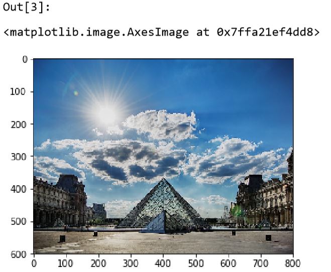
The content image (C) shows the Louvre museum's pyramid surrounded by old Paris buildings, against a sunny sky with a few clouds.
** 3.1.1 - How do you ensure the generated image G matches the content of the image C?**
As we saw in lecture, the earlier (shallower) layers of a ConvNet tend to detect lower-level features such as edges and simple textures, and the later (deeper) layers tend to detect higher-level features such as more complex textures as well as object classes.
We would like the "generated" image G to have similar content as the input image C. Suppose you have chosen some layer's activations to represent the content of an image. In practice, you'll get the most visually pleasing results if you choose a layer in the middle of the network--neither too shallow nor too deep. (After you have finished this exercise, feel free to come back and experiment with using different layers, to see how the results vary.)
So, suppose you have picked one particular hidden layer to use. Now, set the image C as the input to the pretrained VGG network, and run forward propagation. Let \(a^{(C)}\) be the hidden layer activations in the layer you had chosen. (In lecture, we had written this as \(a^{[l](C)}\), but here we'll drop the superscript \([l]\) to simplify the notation.) This will be a \(n_H \times n_W \times n_C\) tensor. Repeat this process with the image G: Set G as the input, and run forward progation. Let \[a^{(G)}\] be the corresponding hidden layer activation. We will define as the content cost function as:
\[J_{content}(C,G) = \frac{1}{4 \times n_H \times n_W \times n_C}\sum _{ \text{all entries}} (a^{(C)} - a^{(G)})^2 \]
Here, $ n_H,n_W $ and $ n_C $ are the height, width and number of channels of the hidden layer you have chosen, and appear in a normalization term in the cost. For clarity, note that $ a^{(C)} $ and $ a^{(G)} $ are the volumes corresponding to a hidden layer's activations. In order to compute the cost $ J_{content}(C,G) $, it might also be convenient to unroll these 3D volumes into a 2D matrix, as shown below. (Technically this unrolling step isn't needed to compute $ J_{content} $, but it will be good practice for when you do need to carry out a similar operation later for computing the style const $ J_{style} $.)

Exercise: Compute the "content cost" using TensorFlow.
Instructions: The 3 steps to implement this function are: 1. Retrieve dimensions from a_G: - To retrieve dimensions from a tensor X, use: X.get_shape().as_list() 2. Unroll a_C and a_G as explained in the picture above - If you are stuck, take a look at Hint1 and Hint2. 3. Compute the content cost: - If you are stuck, take a look at Hint3, Hint4 and Hint5.
1 | #GRADED FUNCTION: compute_content_cost |
What you should remember: - The content cost takes a hidden layer activation of the neural network, and measures how different \(a^{(C)}\) and \(a^{(G)}\) are. - When we minimize the content cost later, this will help make sure \(G\) has similar content as \(C\).
3.2 - Computing the style cost
For our running example, we will use the following style image:
1 | style_image = scipy.misc.imread("images/monet_800600.jpg") |
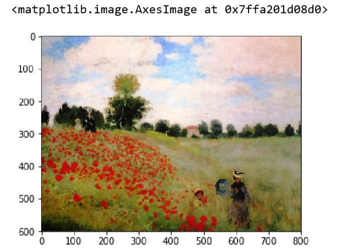
This painting was painted in the style of impressionism.
Lets see how you can now define a "style" const function \(J_{style}(S,G)\).
3.2.1 - Style matrix
The style matrix is also called a "Gram matrix." In linear algebra, the Gram matrix G of a set of vectors \((v_{1},\dots ,v_{n})\) is the matrix of dot products, whose entries are \({\displaystyle G_{ij} = v_{i}^T v_{j} = np.dot(v_{i}, v_{j}) }\). In other words, \(G_{ij}\) compares how similar \(v_i\) is to \(v_j\): If they are highly similar, you would expect them to have a large dot product, and thus for \(G_{ij}\) to be large.
Note that there is an unfortunate collision in the variable names used here. We are following common terminology used in the literature, but \(G\) is used to denote the Style matrix (or Gram matrix) as well as to denote the generated image \(G\). We will try to make sure which \(G\) we are referring to is always clear from the context.
In NST, you can compute the Style matrix by multiplying the "unrolled" filter matrix with their transpose:
The result is a matrix of dimension \((n_C,n_C)\) where \(n_C\) is the number of filters. The value \(G_{ij}\) measures how similar the activations of filter \(i\) are to the activations of filter \(j\).
One important part of the gram matrix is that the diagonal elements such as \(G_{ii}\) also measures how active filter \(i\) is. For example, suppose filter \(i\) is detecting vertical textures in the image. Then \(G_{ii}\) measures how common vertical textures are in the image as a whole: If \(G_{ii}\) is large, this means that the image has a lot of vertical texture.
By capturing the prevalence of different types of features (\(G_{ii}\)), as well as how much different features occur together (\(G_{ij}\)), the Style matrix \(G\) measures the style of an image.
Exercise: Using TensorFlow, implement a function that computes the Gram matrix of a matrix A. The formula is: The gram matrix of A is \(G_A = AA^T\). If you are stuck, take a look at Hint 1 and Hint 2.
1 | #GRADED FUNCTION: gram_matrix |
3.2.2 - Style cost
After generating the Style matrix (Gram matrix), your goal will be to minimize the distance between the Gram matrix of the "style" image S and that of the "generated" image G. For now, we are using only a single hidden layer \(a^{[l]}\), and the corresponding style cost for this layer is defined as:
\[ J_{style}^{[l]}(S,G) = \frac{1}{4 \times {n_C}^2 \times (n_H \times n_W)^2} \sum _{i=1}^{n_C}\sum_{j=1}^{n_C}(G^{(S)}_{ij} - G^{(G)}_{ij})^2 \]
where \(G^{(S)}\) and \(G^{(G)}\) are respectively the Gram matrices of the "style" image and the "generated" image, computed using the hidden layer activations for a particular hidden layer in the network.
Exercise: Compute the style cost for a single layer.
Instructions: The 3 steps to implement this function are: 1. Retrieve dimensions from the hidden layer activations a_G: - To retrieve dimensions from a tensor X, use: X.get_shape().as_list() 2. Unroll the hidden layer activations a_S and a_G into 2D matrices, as explained in the picture above. - You may find Hint1 and Hint2 useful. 3. Compute the Style matrix of the images S and G. (Use the function you had previously written.) 4. Compute the Style cost: - You may find Hint3, Hint4 and Hint5 useful.
1 | #GRADED FUNCTION: compute_layer_style_cost |
3.2.3 Style Weights
So far you have captured the style from only one layer. We'll get better results if we "merge" style costs from several different layers. After completing this exercise, feel free to come back and experiment with different weights to see how it changes the generated image \(G\). But for now, this is a pretty reasonable default:
1 |
|
Note: In the inner-loop of the for-loop above, a_G is a tensor and hasn't been evaluated yet. It will be evaluated and updated at each iteration when we run the TensorFlow graph in model_nn() below.
What you should remember: - The style of an image can be represented using the Gram matrix of a hidden layer's activations. However, we get even better results combining this representation from multiple different layers. This is in contrast to the content representation, where usually using just a single hidden layer is sufficient. - Minimizing the style cost will cause the image \(G\) to follow the style of the image \(S\).
3.3 - Defining the total cost to optimize
Finally, let's create a cost function that minimizes both the style and the content cost. The formula is:
\[J(G) = \alpha J_{content}(C,G) + \beta J_{style}(S,G)\]
Exercise: Implement the total cost function which includes both the content cost and the style cost.
1 |
|
What you should remember: - The total cost is a linear combination of the content cost \(J_{content}(C,G)\) and the style cost \(J_{style}(S,G)\) - \(\alpha\) and \(\beta\) are hyperparameters that control the relative weighting between content and style
4 - Solving the optimization problem
Finally, let's put everything together to implement Neural Style Transfer!
Here's what the program will have to do:
1. Create an Interactive Session 2. Load the content image 3. Load the style image 4. Randomly initialize the image to be generated 5. Load the VGG16 model 7. Build the TensorFlow graph: - Run the content image through the VGG16 model and compute the content cost - Run the style image through the VGG16 model and compute the style cost - Compute the total cost - Define the optimizer and the learning rate 8. Initialize the TensorFlow graph and run it for a large number of iterations, updating the generated image at every step.
Lets go through the individual steps in detail.
You've previously implemented the overall cost \(J(G)\). We'll now set up TensorFlow to optimize this with respect to \(G\). To do so, your program has to reset the graph and use an "Interactive Session". Unlike a regular session, the "Interactive Session" installs itself as the default session to build a graph. This allows you to run variables without constantly needing to refer to the session object, which simplifies the code.
Lets start the interactive session.
1 | #Reset the graph |
Let's load, reshape, and normalize our "content" image (the Louvre museum picture):
1 |
|
Let's load, reshape and normalize our "style" image (Claude Monet's painting):
1 |
|
Now, we initialize the "generated" image as a noisy image created from the content_image. By initializing the pixels of the generated image to be mostly noise but still slightly correlated with the content image, this will help the content of the "generated" image more rapidly match the content of the "content" image. (Feel free to look in nst_utils.py to see the details of generate_noise_image(...); to do so, click "File-->Open..." at the upper-left corner of this Jupyter notebook.)
1 |
|
Next, as explained in part (2), let's load the VGG16 model.
1 |
|
To get the program to compute the content cost, we will now assign a_C and a_G to be the appropriate hidden layer activations. We will use layer conv4_2 to compute the content cost. The code below does the following:
- Assign the content image to be the input to the VGG model.
- Set a_C to be the tensor giving the hidden layer activation for layer "conv4_2".
- Set a_G to be the tensor giving the hidden layer activation for the same layer.
- Compute the content cost using a_C and a_G.
1 | #Assign the content image to be the input of the VGG model. |
Note: At this point, a_G is a tensor and hasn't been evaluated. It will be evaluated and updated at each iteration when we run the Tensorflow graph in model_nn() below.
1 | # Assign the input of the model to be the "style" image |
Exercise: Now that you have J_content and J_style, compute the total cost J by calling total_cost(). Use alpha = 10 and beta = 40.
1 | ##### START CODE HERE ### (1 line) |
You'd previously learned how to set up the Adam optimizer in TensorFlow. Lets do that here, using a learning rate of 2.0. See reference
1 | # define optimizer (1 line) |
Exercise: Implement the model_nn() function which initializes the variables of the tensorflow graph, assigns the input image (initial generated image) as the input of the VGG16 model and runs the train_step for a large number of steps.
1 | def model_nn(sess, input_image, num_iterations = 200): |
Run the following cell to generate an artistic image. It should take about 3min on CPU for every 20 iterations but you start observing attractive results after ≈140 iterations. Neural Style Transfer is generally trained using GPUs.
You're done! After running this, in the upper bar of the notebook click on "File" and then "Open". Go to the "/output" directory to see all the saved images. Open "generated_image" to see the generated image! :)
You should see something the image presented below on the right:
We didn't want you to wait too long to see an initial result, and so had set the hyperparameters accordingly. To get the best looking results, running the optimization algorithm longer (and perhaps with a smaller learning rate) might work better. After completing and submitting this assignment, we encourage you to come back and play more with this notebook, and see if you can generate even better looking images.
Here are few other examples:
- The beautiful ruins of the ancient city of Persepolis (Iran) with the style of Van Gogh (The Starry Night)

- The tomb of Cyrus the great in Pasargadae with the style of a Ceramic Kashi from Ispahan.

- A scientific study of a turbulent fluid with the style of a abstract blue fluid painting.

5 - Test with your own image (Optional/Ungraded)
Finally, you can also rerun the algorithm on your own images!
To do so, go back to part 4 and change the content image and style image with your own pictures. In detail, here's what you should do:
- Click on "File -> Open" in the upper tab of the notebook
- Go to "/images" and upload your images (requirement: (WIDTH = 300, HEIGHT = 225)), rename them "my_content.png" and "my_style.png" for example.
- Change the code in part (3.4) from : to:
1
2content_image = scipy.misc.imread("images/louvre.jpg")
style_image = scipy.misc.imread("images/claude-monet.jpg")1
2content_image = scipy.misc.imread("images/my_content.jpg")
style_image = scipy.misc.imread("images/my_style.jpg") - Rerun the cells (you may need to restart the Kernel in the upper tab of the notebook).
You can also tune your hyperparameters: - Which layers are responsible for representing the style? STYLE_LAYERS - How many iterations do you want to run the algorithm? num_iterations - What is the relative weighting between content and style? alpha/beta
6 - Conclusion
Great job on completing this assignment! You are now able to use Neural Style Transfer to generate artistic images. This is also your first time building a model in which the optimization algorithm updates the pixel values rather than the neural network's parameters. Deep learning has many different types of models and this is only one of them!
What you should remember: - Neural Style Transfer is an algorithm that given a content image C and a style image S can generate an artistic image - It uses representations (hidden layer activations) based on a pretrained ConvNet. - The content cost function is computed using one hidden layer's activations. - The style cost function for one layer is computed using the Gram matrix of that layer's activations. The overall style cost function is obtained using several hidden layers. - Optimizing the total cost function results in synthesizing new images.
This was the final programming exercise of this course. Congratulations--you've finished all the programming exercises of this course on Convolutional Networks! We hope to also see you in Course 5, on Sequence models!
References:
The Neural Style Transfer algorithm was due to Gatys et al. (2015). Harish Narayanan and Github user "log0" also have highly readable write-ups from which we drew inspiration. The pre-trained network used in this implementation is a VGG network, which is due to Simonyan and Zisserman (2015). Pre-trained weights were from the work of the MathConvNet team.
- Leon A. Gatys, Alexander S. Ecker, Matthias Bethge, (2015). A Neural Algorithm of Artistic Style (https://arxiv.org/abs/1508.06576)
- Harish Narayanan, Convolutional neural networks for artistic style transfer. https://harishnarayanan.org/writing/artistic-style-transfer/
- Log0, TensorFlow Implementation of "A Neural Algorithm of Artistic Style". http://www.chioka.in/tensorflow-implementation-neural-algorithm-of-artistic-style
- Karen Simonyan and Andrew Zisserman (2015). Very deep convolutional networks for large-scale image recognition (https://arxiv.org/pdf/1409.1556.pdf)
- MatConvNet. http://www.vlfeat.org/matconvnet/pretrained/