coursera-deeplearning-ai-c4-week3

课程笔记

本周课程主要介绍当前计算机视觉领域最热门的领域：目标检测（Object detection），介绍目标检测的相关概念和基础算法，以及常用的一些网络，包括：

• 目标检测的概念
• 标记点检测（Landmark detection）
• 滑动窗口(Sliding windows)
• 非最大抑制值（non-max suppression）算法
• IOU（intersection over union，交并比）算法
• YOLO网络
• 锚框（Anchor box）

学习目标

• Understand the challenges of Object Localization, Object Detection and Landmark Finding
• Understand and implement non-max suppression
• Understand and implement intersection over union
• Understand how we label a dataset for an object detection application
• Remember the vocabulary of object detection (landmark, anchor, bounding box, grid, ...)

Detection algorithms

Object Localization

分类并定位: 不仅仅要识别出, 并且算法也负责生成一个边框，标出物体的位置。

对象检测， 如何检测在一张图片里的多个对象，并且能够把它们全部检测出来并且定位它们。

对于图像分类 和分类并定位问题，通常只有一个对象。 相比之下，在对象检测问题中，可能会有很多对象。

Landmark Detection

landmark检测是指对图片中的物体的特征点进行检测，比如人脸，标记出人脸上的特征点，如眼角、嘴角、鼻子、下巴等。或者人体特征，如手臂、腿、胸、头等。

Object Detection

目标检测，在深度学习没有兴起之前的做法是，比如要检测车，先训练一个小网络，检测一副小图片中是否包含车。

然后在要检测的图片中，通过下图滑动窗口的方式，在大图片中有个小窗口一直滑动，然后使用网络判断小窗口中是否有车，从而找到车的位置。为了检测的更准确，需要大小不同的几个窗口来进行滑动。

这种方法的缺点是，如果窗口多且滑动步长小，虽然检测精确，但是计算量很大；如果窗口少且滑动步长大，则检测精度不够。不能很好的解决目标检测的问题。

下面通过卷积的方式解决此问题。

Convolutional Implementation of Sliding Windows

首先讲一下，如何把全连接层转换为卷积层进行计算。为下面的用卷积实现滑动窗口做铺垫。

下图中，把上面的全连接层替换为下面的卷积层，后面的全连接全部用卷积替换，可以得到同样的计算结果。

最上面一行，一个14*14的窗口，计算出一个结果，中间一行，输入是16*16，可以划分4个14*14的窗口，经过计算后得到4个结果。这样就可以实现类似滑动窗口的效果，而且大部分计算都是共享的，可以节省大部分的计算量。

同样，最后一行的输入更大，可以划分更多的小窗口，得到更多的结果。

Bounding Box Predictions（边界框预测）

通过前面讲到的滑动窗口目标检测，有时候无法得到精确的预测，因为窗口的大小和位置是固定，而目标出现的位置比较随机。

YOLO(You Only Look Once)算法可以解决此问题，而且速度很快。

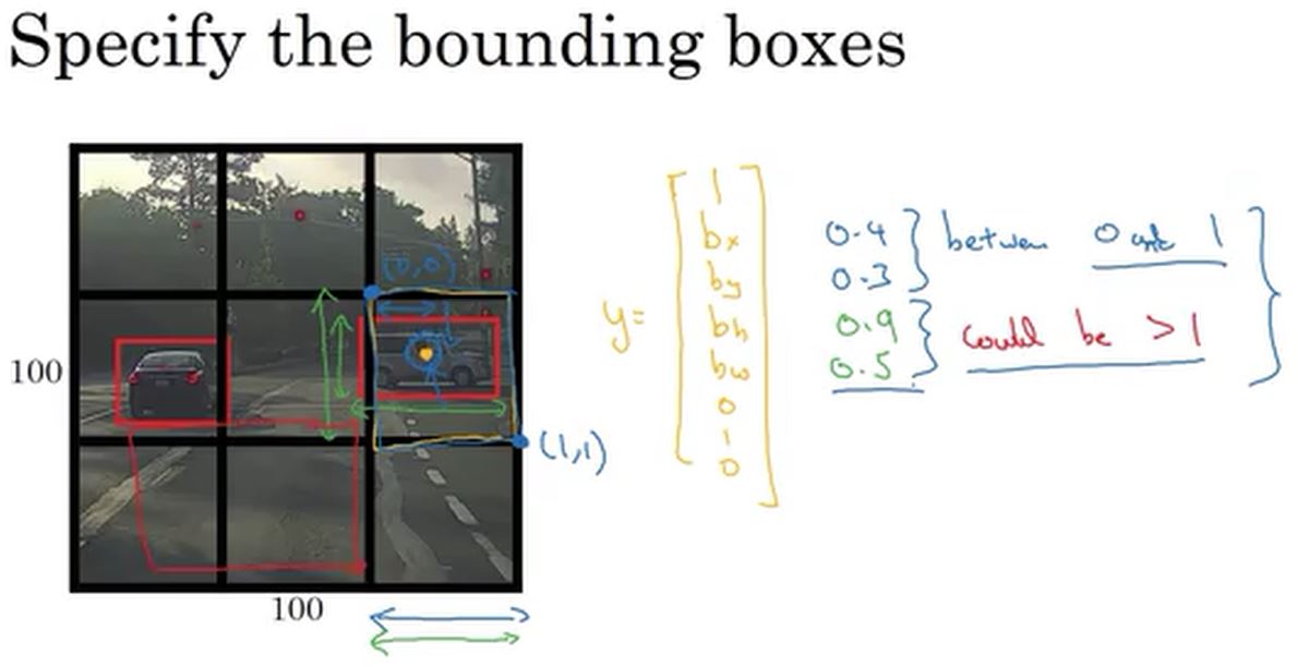
yolo算法的做法是，把输入的图像分割为3×3的窗口（这儿为了讲解方便，使用3×3，实际应用中，是19×19或者其他的划分）。每个窗口对应一个label，label的形式如下图所示，\(p_c\)表示窗口中是否含有目标，然后下面4个值是目标的位置信息，后面3个是对应目标的种类（这儿只检测三种类型的目标，汽车/行人/摩托车）。比如，下图中，9个小窗口，第4个和第6个窗口中包含汽车，则\(p_c = 1\)，其他窗口不含目标，\(p_c = 0\)。

训练集中，每个示例都是一副图片，对应的label和下图中类似。通过卷积和池化等操作，把输入映射到对应的label上。比如下图的示例中，输入是\(100×100×3\)的图片，对应的label是\(3×3×8\)的结果。

算法的优势在于，该神经网络可以精确地输出边界框。在实际操作中，相比这里使用的相对较少的3乘3的网格，可能会使用更精细的网格，可能是19乘19的网格，所以最终会得到19乘19乘8的结果。由于使用了更精细的网格，这会减少同一个网格元中有多个目标物的可能性。值得提醒的是，将目标物分配到网格元中的方式，即先找到目标物的中心点，再根据中心点的位置将它分配到包含该中心点的网格中。所以对于每一个目标物，即使它跨越了多个网格，它也只会被分配给这九个网格元中的一个，或者说这3乘3个网格元中的一个，或者19乘19个网格元中的一个。而使用19乘19的网格的算法，两个目标物的中心，出现在同一个网格元中的概率会稍小。

所以值得注意的有两点：

• 1.这种会直接输出边界框的坐标位置，以及它允许神经网络输出，任意长宽比的边界框，同时输出的坐标位置也更为精确，而不会受限于滑动窗口的步长
• 2.这个算法是通过卷积实现的，不需要在3乘3的网格上执行这个算法9次。这个算法是一整个卷积实现的，只需要用一个卷积网络，所需的计算被大量地共享，这是一个非常有效率的算法。事实上，YOLO算法的一个好处，也是它一直很流行的原因是它是通过卷积实现的，实际上的运行起来非常快，它甚至可以运用在实时的目标识别上。

值得注意的是，YOLO算法中，目标的位置的bx,by,bh,bw是以每个小网格的右上点为参考点。如下图所示。

Intersection Over Union（交并比）

交并比（Intersection Over Union，简称IOU）是用来判断目标检测算法是否有效的算法。它既可以用来评价你的目标检测算法，也可以用于，往目标检测算法中加入其他特征部分，来进一步改善它。

交并比或者说是IoU函数做的是计算两个边界框的交集除以并集的比率。按惯例，或者说计算机视觉领域的原则，如果IoU大于0.5，结果就会被判断为正确的，如果预测的和真实的边界框完美重合了 IoU就会是1。如果你想更严格一些，可以把准确的标准提高，仅当IoU大于等于0.6，或者别的数值。IoU越高，边界框就越准确。

IoU创立的初衷，作为一个评估的方法，来判断目标定位算法是否准确。但更普遍地说，IoU是，两个边界框重叠程度的一个度量值。当有两个框时，可以计算交集，计算并集，然后求两个面积的比值。因此这也是一个方法，来衡量两个框的相近程度。

当讨论非最大值抑制(non-max suppression)时，会用到IoU或者说是交并比。非最大值抑制（non-max suppression） 这个工具可以用来让YOLO的结果变得更理想。

Non-max Suppression

目前所学到的目标检测的问题之一是，算法或许会对同一目标有多次检测。非极大值抑制是一种确保算法只对每个对象得到一个检测结果的方法。

非极大值抑制是如何工作的？

首先，是看一看每个检测结果的相关概率。候选者Pc为一个检测到的概率。首先它取其中最大那个, 如下图中左边的例子是0.9, 意味着 "这是我最自信的检测结果了, 那么让我们标明它, 认为我在这里找到一辆车."

做完这一步, 非极大值抑制再看，所有的剩下的方框以及所有和刚输入的那个结果有着着多重叠的, 有着高IOU值的方形区域得到的产出值将被抑制。就是那二个概率为0,6和0.7的方框。这二个和亮蓝色的方框重叠最多。所以这些将要做抑制。

非极大值意思是将要输出有着最大可能性的分类判断，而抑制那些非最大可能性的邻近的方框。因此叫做非极大值抑制。

过一下这个算法的细节。为了运用非极大值抑制：

• 首先要做的是丢掉所有预测值Pc小于或等于 某个门限的边界框, 例如0.6.
• 接下来, 如果还有剩下的边界框,还没有被去掉或处理的, 将重复地选出有着最大概率最大Pc值的边界框, 将它作为一个预测结果.
• 然后，要丢掉其他剩余边界框, 即那些不被认为是预测结果的, 并且之前也没有被去掉的框。因此丢弃任何“剩余的，同上一步的计算有着着多重叠的, 高IOU值的边框”。
• 需要重复这个过程, 直到每个边界框不是被输出为预测结果, 就是被丢弃掉, 由于它们有着很大的重复或很高的IOU值。和刚刚检测输出的目标检测来作为你检测到的目标相比。

Anchor Boxes

前面的例子中，每个网格都是检测单一目标，但实际应用中，很可能一个网格含有多个目标。下面讲到的Anchor Boxes（锚框）可以解决此问题。

如下图所示，示例图片中，一个网格包含两个目标物体，通过两个锚框，分别对应两个目标。对应的label的大小是3×3×16，分别对应2个锚框检测的结果。

在此之前，每个目标在训练集中，分配在包含这个目标中心点的网格中。有了锚框算法后，每个目标在训练集中，这个目标分配的网格不仅要包含这个目标中心点，还要和对应的锚框有最高的IOU值。

下图是一个示例，对于车这个目标，和锚框2的IOU值更高，所以对应到锚框2的位置，人和锚框1的IOU值更高，对应到锚框1的位置。

还有一些细节，有两个锚框，但是万一同一格子裡有三个物件呢？此算法对这个例子没办法处理好，希望这不会发生，不过如果真有其事，此算法并没有好法子处理。对这种情形，会写某种挑选的机制。 还有，万一有两个物件在同一个格子，但是两个都和同一个锚框的形状一样呢？ 同样地，此算法也无法处理好这情况。如果发生这种情况，可以做一些挑选的机制 (tiebreaking)。希望资料集不会出现这种例子，希望不会常发生。 但实际上，这很少发生。特别是当用19×19，而不只是 3×3 格子，在 361 个格子有两个物件的中心点在同一个格子，的确有这机会，但概率很小。

最后，怎么选择锚框呢？大家曾经是手动挑选，可能设计五或十个锚框，让他们有各种不同形状，看起来能涵盖想侦测的物件种类。 而更进阶的版本，是利用 K-means 算法 (K-平均)： 把两种想侦测的物件的形状集合起来，然后利用k-平均算法，挑选出一些锚框，最具代表性的、让他们能展现出想侦测的、多种各个类别的物件。 不过这种自动选择锚框的方法比较进阶。如果手动挑选各式各样的形状，能够扩展出想侦测的物件形状，想找高的、 瘦的、胖的宽的... 应该也能表现不错。

YOLO Algorithm

把上面学到的东西，组合回 YOLO 算法。

首先是训练。下图中给出了训练集中label的样式。网格划分是3×3，有两个锚框，检测的目标物体是3种类型，那么label的大小是3×3×2×8。

然后是进行预测，预测的结果同样是3×3×2×8的大小。

下图是一个预测后的结果，通过去除低概率的预测值，再通过非最大值抑制算法，得到最终的结果。

(Optional) Region Proposals

Region Proposal(候选区域)在计算机视觉中也非常流行。R-CNN 算法中用到了 Region Proposal,它的意思是，伴随区域的卷积网络或者伴随区域的CNN。这个算法所做的是，它会尝试选取，仅仅是少许有意义的区域，用来进行目标检测。所以，相较于运行每一个移动窗口，可以用选取少许窗口的方式来代替。所用的运行区域候选的方法，是通过运行所谓的分割算法来实现的。

下图是R-CNN算法及其进阶版本的介绍。

编程练习

Autonomous driving - Car detection

Welcome to your week 3 programming assignment. You will learn about object detection using the very powerful YOLO model. Many of the ideas in this notebook are described in the two YOLO papers: Redmon et al., 2016 (https://arxiv.org/abs/1506.02640) and Redmon and Farhadi, 2016 (https://arxiv.org/abs/1612.08242).

You will learn to: - Use object detection on a car detection dataset - Deal with bounding boxes

Run the following cell to load the packages and dependencies that are going to be useful for your journey!

import argparse
import os
import matplotlib.pyplot as plt
from matplotlib.pyplot import imshow
import scipy.io
import scipy.misc
import numpy as np
import pandas as pd
import PIL
import tensorflow as tf
from keras import backend as K
from keras.layers import Input, Lambda, Conv2D
from keras.models import load_model, Model
from yolo_utils import read_classes, read_anchors, generate_colors, preprocess_image, draw_boxes, scale_boxes
from yad2k.models.keras_yolo import yolo_head, yolo_boxes_to_corners, preprocess_true_boxes, yolo_loss, yolo_body

get_ipython().magic('matplotlib inline')

Important Note: As you can see, we import Keras's backend as K. This means that to use a Keras function in this notebook, you will need to write: K.function(...).

1 - Problem Statement

You are working on a self-driving car. As a critical component of this project, you'd like to first build a car detection system. To collect data, you've mounted a camera to the hood (meaning the front) of the car, which takes pictures of the road ahead every few seconds while you drive around.

You've gathered all these images into a folder and have labelled them by drawing bounding boxes around every car you found. Here's an example of what your bounding boxes look like.

If you have 80 classes that you want YOLO to recognize, you can represent the class label \(c\) either as an integer from 1 to 80, or as an 80-dimensional vector (with 80 numbers) one component of which is 1 and the rest of which are 0. The video lectures had used the latter representation; in this notebook, we will use both representations, depending on which is more convenient for a particular step.

In this exercise, you will learn how YOLO works, then apply it to car detection. Because the YOLO model is very computationally expensive to train, we will load pre-trained weights for you to use.

2 - YOLO

YOLO ("you only look once") is a popular algoritm because it achieves high accuracy while also being able to run in real-time. This algorithm "only looks once" at the image in the sense that it requires only one forward propagation pass through the network to make predictions. After non-max suppression, it then outputs recognized objects together with the bounding boxes.

2.1 - Model details

First things to know: - The input is a batch of images of shape (m, 608, 608, 3) - The output is a list of bounding boxes along with the recognized classes. Each bounding box is represented by 6 numbers \((p_c, b_x, b_y, b_h, b_w, c)\) as explained above. If you expand \(c\) into an 80-dimensional vector, each bounding box is then represented by 85 numbers.

We will use 5 anchor boxes. So you can think of the YOLO architecture as the following: IMAGE (m, 608, 608, 3) -> DEEP CNN -> ENCODING (m, 19, 19, 5, 85).

Lets look in greater detail at what this encoding represents.

If the center/midpoint of an object falls into a grid cell, that grid cell is responsible for detecting that object.

Since we are using 5 anchor boxes, each of the 19 x19 cells thus encodes information about 5 boxes. Anchor boxes are defined only by their width and height.

For simplicity, we will flatten the last two last dimensions of the shape (19, 19, 5, 85) encoding. So the output of the Deep CNN is (19, 19, 425).

Now, for each box (of each cell) we will compute the following elementwise product and extract a probability that the box contains a certain class.

Here's one way to visualize what YOLO is predicting on an image: - For each of the 19x19 grid cells, find the maximum of the probability scores (taking a max across both the 5 anchor boxes and across different classes). - Color that grid cell according to what object that grid cell considers the most likely.

Doing this results in this picture:

Note that this visualization isn't a core part of the YOLO algorithm itself for making predictions; it's just a nice way of visualizing an intermediate result of the algorithm.

Another way to visualize YOLO's output is to plot the bounding boxes that it outputs. Doing that results in a visualization like this:

In the figure above, we plotted only boxes that the model had assigned a high probability to, but this is still too many boxes. You'd like to filter the algorithm's output down to a much smaller number of detected objects. To do so, you'll use non-max suppression. Specifically, you'll carry out these steps: - Get rid of boxes with a low score (meaning, the box is not very confident about detecting a class) - Select only one box when several boxes overlap with each other and detect the same object.

2.2 - Filtering with a threshold on class scores

You are going to apply a first filter by thresholding. You would like to get rid of any box for which the class "score" is less than a chosen threshold.

The model gives you a total of 19x19x5x85 numbers, with each box described by 85 numbers. It'll be convenient to rearrange the (19,19,5,85) (or (19,19,425)) dimensional tensor into the following variables:
- box_confidence: tensor of shape \((19 \times 19, 5, 1)\) containing \(p_c\) (confidence probability that there's some object) for each of the 5 boxes predicted in each of the 19x19 cells. - boxes: tensor of shape \((19 \times 19, 5, 4)\) containing \((b_x, b_y, b_h, b_w)\) for each of the 5 boxes per cell. - box_class_probs: tensor of shape \((19 \times 19, 5, 80)\) containing the detection probabilities \((c_1, c_2, ... c_{80})\) for each of the 80 classes for each of the 5 boxes per cell.

Exercise: Implement yolo_filter_boxes(). 1. Compute box scores by doing the elementwise product as described in Figure 4. The following code may help you choose the right operator:

a = np.random.randn(19*19, 5, 1)
b = np.random.randn(19*19, 5, 80)
c = a * b # shape of c will be (19*19, 5, 80)

2. For each box, find: - the index of the class with the maximum box score (Hint) (Be careful with what axis you choose; consider using axis=-1) - the corresponding box score (Hint) (Be careful with what axis you choose; consider using axis=-1) 3. Create a mask by using a threshold. As a reminder: ([0.9, 0.3, 0.4, 0.5, 0.1] < 0.4) returns: [False, True, False, False, True]. The mask should be True for the boxes you want to keep. 4. Use TensorFlow to apply the mask to box_class_scores, boxes and box_classes to filter out the boxes we don't want. You should be left with just the subset of boxes you want to keep. (Hint)

Reminder: to call a Keras function, you should use K.function(...).

#GRADED FUNCTION: yolo_filter_boxes

def yolo_filter_boxes(box_confidence, boxes, box_class_probs, threshold = .6):
    """Filters YOLO boxes by thresholding on object and class confidence.
    
    Arguments:
    box_confidence -- tensor of shape (19, 19, 5, 1)
    boxes -- tensor of shape (19, 19, 5, 4)
    box_class_probs -- tensor of shape (19, 19, 5, 80)
    threshold -- real value, if [ highest class probability score < threshold], then get rid of the corresponding box
    
    Returns:
    scores -- tensor of shape (None,), containing the class probability score for selected boxes
    boxes -- tensor of shape (None, 4), containing (b_x, b_y, b_h, b_w) coordinates of selected boxes
    classes -- tensor of shape (None,), containing the index of the class detected by the selected boxes
    
    Note: "None" is here because you don't know the exact number of selected boxes, as it depends on the threshold. 
    For example, the actual output size of scores would be (10,) if there are 10 boxes.
    """
    
    # Step 1: Compute box scores
    ### START CODE HERE ### (≈ 1 line)
    box_scores = box_confidence * box_class_probs
    ### END CODE HERE ###
    
    # Step 2: Find the box_classes thanks to the max box_scores, keep track of the corresponding score
    ### START CODE HERE ### (≈ 2 lines)
    box_classes = K.argmax(box_scores, axis=-1)
    box_class_scores = K.max(box_scores, axis=-1)
    ### END CODE HERE ###
    
    # Step 3: Create a filtering mask based on "box_class_scores" by using "threshold". The mask should have the
    # same dimension as box_class_scores, and be True for the boxes you want to keep (with probability >= threshold)
    ### START CODE HERE ### (≈ 1 line)
    filtering_mask = box_class_scores >= threshold
    ### END CODE HERE ###
    
    # Step 4: Apply the mask to scores, boxes and classes
    ### START CODE HERE ### (≈ 3 lines)
    scores = tf.boolean_mask(box_class_scores, filtering_mask)
    boxes = tf.boolean_mask(boxes, filtering_mask)
    classes = tf.boolean_mask(box_classes, filtering_mask)
    ### END CODE HERE ###
    
    return scores, boxes, classes

2.3 - Non-max suppression

Even after filtering by thresholding over the classes scores, you still end up a lot of overlapping boxes. A second filter for selecting the right boxes is called non-maximum suppression (NMS).

Non-max suppression uses the very important function called "Intersection over Union", or IoU.

1 2 3 4 5 6 7 8 9 10 11 12 13 14 15 16 17 18 19 20 21 22 23 24 25 26 27 28 29 30 31 32 33

#GRADED FUNCTION: iou def iou(box1, box2): """Implement the intersection over union (IoU) between box1 and box2      Arguments: box1 -- first box, list object with coordinates (x1, y1, x2, y2)     box2 -- second box, list object with coordinates (x1, y1, x2, y2)     """ # Calculate the (y1, x1, y2, x2) coordinates of the intersection of box1 and box2. Calculate its Area. ### START CODE HERE ### (≈ 5 lines) xi1 = max(box1[0],box2[0]) yi1 = max(box1[1],box2[1]) xi2 = min(box1[2],box2[2]) yi2 = min(box1[3],box2[3]) inter_area = (yi2-yi1)*(xi2-xi1) if (max(yi2-yi1,0) > 0 and max(xi2-xi1,0) > 0) else 0 ### END CODE HERE ###     # Calculate the Union area by using Formula: Union(A,B) = A + B - Inter(A,B) ### START CODE HERE ### (≈ 3 lines) box1_area = (box1[3] -box1[1]) * (box1[2] -box1[0]) box2_area = (box2[3] -box2[1]) * (box2[2] -box2[0]) union_area = box1_area + box2_area - inter_area ### END CODE HERE ### # compute the IoU ### START CODE HERE ### (≈ 1 line) iou = 1.0 * inter_area / union_area ### END CODE HERE ### return iou

<p>You are now ready to implement non-max suppression. The key steps are: 1. Select the box that has the highest score. 2. Compute its overlap with all other boxes, and remove boxes that overlap it more than <code>iou_threshold</code>. 3. Go back to step 1 and iterate until there">

What you should remember: - YOLO is a state-of-the-art object detection model that is fast and accurate - It runs an input image through a CNN which outputs a 19x19x5x85 dimensional volume. - The encoding can be seen as a grid where each of the 19x19 cells contains information about 5 boxes. - You filter through all the boxes using non-max suppression. Specifically: - Score thresholding on the probability of detecting a class to keep only accurate (high probability) boxes - Intersection over Union (IoU) thresholding to eliminate overlapping boxes - Because training a YOLO model from randomly initialized weights is non-trivial and requires a large dataset as well as lot of computation, we used previously trained model parameters in this exercise. If you wish, you can also try fine-tuning the YOLO model with your own dataset, though this would be a fairly non-trivial exercise.

References: The ideas presented in this notebook came primarily from the two YOLO papers. The implementation here also took significant inspiration and used many components from Allan Zelener's github repository. The pretrained weights used in this exercise came from the official YOLO website. - Joseph Redmon, Santosh Divvala, Ross Girshick, Ali Farhadi - You Only Look Once: Unified, Real-Time Object Detection (2015) - Joseph Redmon, Ali Farhadi - YOLO9000: Better, Faster, Stronger (2016) - Allan Zelener - YAD2K: Yet Another Darknet 2 Keras - The official YOLO website (https://pjreddie.com/darknet/yolo/)

Car detection dataset:
The Drive.ai Sample Dataset (provided by drive.ai) is licensed under a Creative Commons Attribution 4.0 International License. We are especially grateful to Brody Huval, Chih Hu and Rahul Patel for collecting and providing this dataset.