课程笔记
本周课程从边缘检测讲起,引出卷积的概念,并讲到了卷积中的padding、pooling等操作,要点: - 边缘检测 - 卷积的实现 - padding - pooling - stride
学习目标:
- Understand the convolution operation
- Understand the pooling operation
- Remember the vocabulary used in convolutional neural network (padding, stride, filter, ...)
- Build a convolutional neural network for image multi-class classification
Convolutional Neural Networks
Computer Vision
计算机视觉的应用:
- Image Classification
- Object detection
- Image Style Transfer
Edge Detection Example
通过特定的filter,可以检测出特定的边缘。比如,下图中的filter可以检测出垂直方向的边缘。

More Edge Detection

在深度学习领域,要通过训练学习的方式,学习得到filter来检测不同的边缘。
Padding
上面给的filter,会把结果图像的尺寸变小,所以通过padding操作,在输入图像边缘填充的方式,使得原图像变大,以保持输出尺寸和原图像大小一致。
输出图像的尺寸计算公式为:$ n - f +1 $
加入padding后,输出图像的尺寸计算公式为:$ n + 2p - f + 1 $
为了使输出图像尺寸保持不变,即$ n + 2p - f + 1 = n $,所以
\[ p = \frac{ f - 1 }{2} \]
有两种padding方式:
- VALID: 不进行padding,输出图像的尺寸计算公式为:$ n - f +1 $
- SAME: 进行padding,大小为:\[ p = \frac{ f - 1 }{2} \]
注:深度学习领域,一般情况下f取值为奇数,比如1、3、5、7等。否则会出现不对称填充。
Tensorflow中,VALID padding的实现如下:
\[ \text{padding along height} = P_h = max((\text{output height}-1)*S_h + F_h - H, 0) \]
\[ \text{padding along width} = P_w = max((\text{output width}-1)*S_w + F_w - W, 0) \]
\[ \text{padding top} = P_t = Floor(\dfrac{P_h}{2}) \qquad \qquad \text{padding left} = P_l = Floor(\dfrac{P_w}{2}) \]
\[ \text{padding bottom} = P_h - P_t \qquad \qquad \text{padding right} = P_w - P_l \]
代码实现为:
For the 'SAME' padding, the output height and width are computed as:
1 | out_height = ceil(float(in_height) / float(strides[1])) |
and the padding on the top and left are computed as:
1 | pad_along_height = max((out_height - 1) * strides[1] + filter_height - in_height, 0) |
For the 'VALID' padding, the output height and width are computed as:
1 | out_height = ceil(float(in_height - filter_height + 1) / float(strides[1])) |
and the padding values are always zero.
Strided Convolutions
步长是卷积核进行计算是每次跳跃的长度。

\[ \text{output width} = \dfrac{W-F_w+2P}{S_w}+1 \]
\[ \text{output height} = \dfrac{H-F_h+2P}{S_h}+1 \]

Convolutions Over Volume
上面讲的卷积是二维的,在正常卷积神经网络中,卷积一般是3维的,也就是多channel的,通过下图可以理解多channel卷积的计算。

上图中,输入是一副图片,3个通道(RGB),filter也对应3个通道,计算后得到一个2维的结果。如果想要结果也是多维的,则需要多个fliter,如下图:

One Layer of a Convolutional Network
卷积层和之前讲到的神经网络的典型计算公式是类似的。
下图是各种卷积层的概念的表达方式:

Simple Convolutional Network Example
下图是一个典型卷积网络的例子:

Types of layer in a convolutional network:
- Convolution
- Pooling
- Fully connected
Pooling Layers

Max Pooling的一个有趣的特性是:它有一套超参,但是它没有任何参数需要学习。没有任何需要梯度相加算法学习的东西,一旦确定了$ f \(和\) s $就确定了计算,而且梯度下降算法不会对其有任何改变。
上面卷积层计算输出size的公式同样在这里适用。
还有一种是Average Pooling,就是求filter*filter内的平均值。相比来说,Max Pooling用的更多。
Pooling层的超参数有如下三个:
- f : filter size
- s : stride
- Max or average pooling
不需要通过学习即可确定。
CNN Example
下图是一个卷积神经网络的示例,是基于LeNet-5网络改造的。

注: LeNet-5网络是Yann LeCun在1998年设计的用于手写数字识别的卷积神经网络,当年美国大多数银行就是用它来识别支票上面的手写数字的,它是早期卷积神经网络中最有代表性的实验系统之一。可参考:http://yann.lecun.com/exdb/lenet/ LeNet-5的数据集是MNIST,一般也是各种深度学习框架的入门示例,学习起来很好理解,也很简单,作为入门的示例非常好。 这个网站http://scs.ryerson.ca/~aharley/vis/conv/做了一个3D展示LeNet-5网络每一层的效果,看起来很清晰,推荐。
下图是上面的LeNet-5网络的每一层的参数个数表,可以看出,卷积层的参数相比于全连接层是非常少的,这也是卷积层的优势所在。

关于超参数组选择的建议:
不要试着创造你自己的超参数组,而是查看文献,看看其他人使用的超参数,从中选一组适用于其他人的超参数,很可能它也适用于你的应用。
通常随着神经网络的深入,高度\(n_h\)和宽度\(n_w\)会减小。然而通道数量会增加,最后是全连通网络层。另一类常见的神经网络模型是,一个或多个卷积层接着一层池化层,再接着一个或多个卷积层叠加一层池化层,然后叠加几层全连接,也许最后还叠加一个Softmax层。
Why Convolutions?
卷积网络有效的原因:
- Parameter sharing(参数共享): A feature detector (such as a vertical edge detector) that’s useful in one part of the image is probably useful in another part of the image.
- Sparsity of connections(稀疏式联系): In each layer, each output value depends only on a small number of inputs.

编程练习
Convolutional Neural Networks: Step by Step
Welcome to Course 4's first assignment! In this assignment, you will implement convolutional (CONV) and pooling (POOL) layers in numpy, including both forward propagation and (optionally) backward propagation.
Notation: - Superscript \([l]\) denotes an object of the \(l^{th}\) layer. - Example: \(a^{[4]}\) is the \(4^{th}\) layer activation. \(W^{[5]}\) and \(b^{[5]}\) are the \(5^{th}\) layer parameters.
- Superscript \((i)\) denotes an object from the \(i^{th}\) example.
- Example: \(x^{(i)}\) is the \(i^{th}\) training example input.
- Lowerscript \(i\) denotes the \(i^{th}\) entry of a vector.
- Example: \(a^{[l]}_i\) denotes the \(i^{th}\) entry of the activations in layer \(l\), assuming this is a fully connected (FC) layer.
- \(n_H\), \(n_W\) and \(n_C\) denote respectively the height, width and number of channels of a given layer. If you want to reference a specific layer \(l\), you can also write \(n_H^{[l]}\), \(n_W^{[l]}\), \(n_C^{[l]}\).
- \(n_{H_{prev}}\), \(n_{W_{prev}}\) and \(n_{C_{prev}}\) denote respectively the height, width and number of channels of the previous layer. If referencing a specific layer \(l\), this could also be denoted \(n_H^{[l-1]}\), \(n_W^{[l-1]}\), \(n_C^{[l-1]}\).
We assume that you are already familiar with numpy and/or have completed the previous courses of the specialization. Let's get started!
1 - Packages
Let's first import all the packages that you will need during this assignment. - numpy is the fundamental package for scientific computing with Python. - matplotlib is a library to plot graphs in Python. - np.random.seed(1) is used to keep all the random function calls consistent. It will help us grade your work.
1 | import numpy as np |
2 - Outline of the Assignment
You will be implementing the building blocks of a convolutional neural network! Each function you will implement will have detailed instructions that will walk you through the steps needed:
- Convolution functions, including:
- Zero Padding
- Convolve window
- Convolution forward
- Convolution backward (optional)
- Pooling functions, including:
- Pooling forward
- Create mask
- Distribute value
- Pooling backward (optional)
This notebook will ask you to implement these functions from scratch in numpy. In the next notebook, you will use the TensorFlow equivalents of these functions to build the following model:

Note that for every forward function, there is its corresponding backward equivalent. Hence, at every step of your forward module you will store some parameters in a cache. These parameters are used to compute gradients during backpropagation.
3 - Convolutional Neural Networks
Although programming frameworks make convolutions easy to use, they remain one of the hardest concepts to understand in Deep Learning. A convolution layer transforms an input volume into an output volume of different size, as shown below.

In this part, you will build every step of the convolution layer. You will first implement two helper functions: one for zero padding and the other for computing the convolution function itself.
3.1 - Zero-Padding
Zero-padding adds zeros around the border of an image:
 with a padding of 2.")
The main benefits of padding are the following:
It allows you to use a CONV layer without necessarily shrinking the height and width of the volumes. This is important for building deeper networks, since otherwise the height/width would shrink as you go to deeper layers. An important special case is the "same" convolution, in which the height/width is exactly preserved after one layer.
It helps us keep more of the information at the border of an image. Without padding, very few values at the next layer would be affected by pixels as the edges of an image.
Exercise: Implement the following function, which pads all the images of a batch of examples X with zeros. Use np.pad. Note if you want to pad the array "a" of shape \((5,5,5,5,5)\) with pad = 1 for the 2nd dimension, pad = 3 for the 4th dimension and pad = 0 for the rest, you would do:
1 | a = np.pad(a, ((0,0), (1,1), (0,0), (3,3), (0,0)), 'constant', constant_values = (..,..)) |
1 | #RADED FUNCTION: zero_pad |
3.2 - Single step of convolution
In this part, implement a single step of convolution, in which you apply the filter to a single position of the input. This will be used to build a convolutional unit, which:
- Takes an input volume
- Applies a filter at every position of the input
- Outputs another volume (usually of different size)
")
In a computer vision application, each value in the matrix on the left corresponds to a single pixel value, and we convolve a 3x3 filter with the image by multiplying its values element-wise with the original matrix, then summing them up and adding a bias. In this first step of the exercise, you will implement a single step of convolution, corresponding to applying a filter to just one of the positions to get a single real-valued output.
Later in this notebook, you'll apply this function to multiple positions of the input to implement the full convolutional operation.
Exercise: Implement conv_single_step(). Hint.
1 | # GRADED FUNCTION: conv_single_step |
3.3 - Convolutional Neural Networks - Forward pass
In the forward pass, you will take many filters and convolve them on the input. Each 'convolution' gives you a 2D matrix output. You will then stack these outputs to get a 3D volume:

Exercise: Implement the function below to convolve the filters W on an input activation A_prev. This function takes as input A_prev, the activations output by the previous layer (for a batch of m inputs), F filters/weights denoted by W, and a bias vector denoted by b, where each filter has its own (single) bias. Finally you also have access to the hyperparameters dictionary which contains the stride and the padding.
Hint: 1. To select a 2x2 slice at the upper left corner of a matrix "a_prev" (shape (5,5,3)), you would do: 1
a_slice_prev = a_prev[0:2,0:2,:]
a_slice_prev below, using the start/end indexes you will define. 2. To define a_slice you will need to first define its corners vert_start, vert_end, horiz_start and horiz_end. This figure may be helpful for you to find how each of the corner can be defined using h, w, f and s in the code below.
. This figure shows only a single channel")
Reminder: The formulas relating the output shape of the convolution to the input shape is: \[ n_H = \lfloor \frac{n_{H_{prev}} - f + 2 \times pad}{stride} \rfloor +1 \]
\[ n_W = \lfloor \frac{n_{W_{prev}} - f + 2 \times pad}{stride} \rfloor +1 \]
\[ n_C = \text{number of filters used in the convolution}\]
For this exercise, we won't worry about vectorization, and will just implement everything with for-loops.
1 | # GRADED FUNCTION: conv_forward |
Finally, CONV layer should also contain an activation, in which case we would add the following line of code:
1 | # Convolve the window to get back one output neuron |
You don't need to do it here.
4 - Pooling layer
The pooling (POOL) layer reduces the height and width of the input. It helps reduce computation, as well as helps make feature detectors more invariant to its position in the input. The two types of pooling layers are:
Max-pooling layer: slides an (\(f, f\)) window over the input and stores the max value of the window in the output.
Average-pooling layer: slides an (\(f, f\)) window over the input and stores the average value of the window in the output.


These pooling layers have no parameters for backpropagation to train. However, they have hyperparameters such as the window size \(f\). This specifies the height and width of the fxf window you would compute a max or average over.
4.1 - Forward Pooling
Now, you are going to implement MAX-POOL and AVG-POOL, in the same function.
Exercise: Implement the forward pass of the pooling layer. Follow the hints in the comments below.
Reminder: As there's no padding, the formulas binding the output shape of the pooling to the input shape is:
\[ n_H = \lfloor \frac{n_{H_{prev}} - f}{stride} \rfloor +1 \]
\[ n_W = \lfloor \frac{n_{W_{prev}} - f}{stride} \rfloor +1 \]
\[ n_C = n_{C_{prev}}\]
1 | #GRADED FUNCTION: pool_forward |
Congratulations! You have now implemented the forward passes of all the layers of a convolutional network.
The remainer of this notebook is optional, and will not be graded.
5 - Backpropagation in convolutional neural networks (OPTIONAL / UNGRADED)
In modern deep learning frameworks, you only have to implement the forward pass, and the framework takes care of the backward pass, so most deep learning engineers don't need to bother with the details of the backward pass. The backward pass for convolutional networks is complicated. If you wish however, you can work through this optional portion of the notebook to get a sense of what backprop in a convolutional network looks like.
When in an earlier course you implemented a simple (fully connected) neural network, you used backpropagation to compute the derivatives with respect to the cost to update the parameters. Similarly, in convolutional neural networks you can to calculate the derivatives with respect to the cost in order to update the parameters. The backprop equations are not trivial and we did not derive them in lecture, but we briefly presented them below.
5.1 - Convolutional layer backward pass
Let's start by implementing the backward pass for a CONV layer.
5.1.1 - Computing dA
This is the formula for computing \(dA\) with respect to the cost for a certain filter \(W_c\) and a given training example:
\[ dA += \sum _{h=0} ^{n_H} \sum_{w=0} ^{n_W} W_c \times dZ_{hw} \]
Where \(W_c\) is a filter and \(dZ_{hw}\) is a scalar corresponding to the gradient of the cost with respect to the output of the conv layer \(Z\) at the \(h^{th}\) row and wth column (corresponding to the dot product taken at the ith stride left and jth stride down). Note that at each time, we multiply the the same filter \(W_c\) by a different dZ when updating \(dA\). We do so mainly because when computing the forward propagation, each filter is dotted and summed by a different a_slice. Therefore when computing the backprop for \(dA\), we are just adding the gradients of all the a_slices.
In code, inside the appropriate for-loops, this formula translates into:
1 | da_prev_pad[vert_start:vert_end, horiz_start:horiz_end, :] += W[:,:,:,c] * dZ[i, h, w, c] |
5.1.2 - Computing dW
This is the formula for computing \(dW_c\) (\(dW_c\) is the derivative of one filter) with respect to the loss:
\[ dW_c += \sum _{h=0} ^{n_H} \sum_{w=0} ^ {n_W} a_{slice} \times dZ_{hw} \]
Where $ a_{slice} $ corresponds to the slice which was used to generate the acitivation $ Z_{ij} $. Hence, this ends up giving us the gradient for $ W $ with respect to that slice. Since it is the same $ W $, we will just add up all such gradients to get $ dW $.
In code, inside the appropriate for-loops, this formula translates into: 1
dW[:,:,:,c] += a_slice * dZ[i, h, w, c]
5.1.3 - Computing db
This is the formula for computing \(db\) with respect to the cost for a certain filter \(W_c\):
\[ db = \sum_h \sum_w dZ_{hw} \]
As you have previously seen in basic neural networks, db is computed by summing \(dZ\). In this case, you are just summing over all the gradients of the conv output (Z) with respect to the cost.
In code, inside the appropriate for-loops, this formula translates into: 1
db[:,:,:,c] += dZ[i, h, w, c]
Exercise: Implement the conv_backward function below. You should sum over all the training examples, filters, heights, and widths. You should then compute the derivatives using formulas 1, 2 and 3 above.
1 | def conv_backward(dZ, cache): |
5.2 Pooling layer - backward pass
Next, let's implement the backward pass for the pooling layer, starting with the MAX-POOL layer. Even though a pooling layer has no parameters for backprop to update, you still need to backpropagation the gradient through the pooling layer in order to compute gradients for layers that came before the pooling layer.
5.2.1 Max pooling - backward pass
Before jumping into the backpropagation of the pooling layer, you are going to build a helper function called create_mask_from_window() which does the following:
\[ X = \begin{bmatrix} 1 && 3 \\ 4 && 2 \end{bmatrix} \quad \rightarrow \quad M =\begin{bmatrix} 0 && 0 \\ 1 && 0 \end{bmatrix}\]
As you can see, this function creates a "mask" matrix which keeps track of where the maximum of the matrix is. True (1) indicates the position of the maximum in X, the other entries are False (0). You'll see later that the backward pass for average pooling will be similar to this but using a different mask.
Exercise: Implement create_mask_from_window(). This function will be helpful for pooling backward. Hints: - np.max() may be helpful. It computes the maximum of an array. - If you have a matrix X and a scalar x: A = (X == x) will return a matrix A of the same size as X such that: 1
2A[i,j] = True if X[i,j] = x
A[i,j] = False if X[i,j] != x
1 | def create_mask_from_window(x): |
Why do we keep track of the position of the max? It's because this is the input value that ultimately influenced the output, and therefore the cost. Backprop is computing gradients with respect to the cost, so anything that influences the ultimate cost should have a non-zero gradient. So, backprop will "propagate" the gradient back to this particular input value that had influenced the cost.
5.2.2 - Average pooling - backward pass
In max pooling, for each input window, all the "influence" on the output came from a single input value--the max. In average pooling, every element of the input window has equal influence on the output. So to implement backprop, you will now implement a helper function that reflects this.
For example if we did average pooling in the forward pass using a 2x2 filter, then the mask you'll use for the backward pass will look like: \[ dZ = 1 \quad \rightarrow \quad dZ =\begin{bmatrix} 1/4 && 1/4 \\ 1/4 && 1/4 \end{bmatrix}\]
This implies that each position in the \(dZ\) matrix contributes equally to output because in the forward pass, we took an average.
Exercise: Implement the function below to equally distribute a value dz through a matrix of dimension shape. Hint
1 | def distribute_value(dz, shape): |
5.2.3 Putting it together: Pooling backward
You now have everything you need to compute backward propagation on a pooling layer.
Exercise: Implement the pool_backward function in both modes ("max" and "average"). You will once again use 4 for-loops (iterating over training examples, height, width, and channels). You should use an if/elif statement to see if the mode is equal to 'max' or 'average'. If it is equal to 'average' you should use the distribute_value() function you implemented above to create a matrix of the same shape as a_slice. Otherwise, the mode is equal to 'max', and you will create a mask with create_mask_from_window() and multiply it by the corresponding value of dZ.
1 | def pool_backward(dA, cache, mode = "max"): |
Congratulations !
Congratulation on completing this assignment. You now understand how convolutional neural networks work. You have implemented all the building blocks of a neural network. In the next assignment you will implement a ConvNet using TensorFlow.
Convolutional Neural Networks: Application
Welcome to Course 4's second assignment! In this notebook, you will:
- Implement helper functions that you will use when implementing a TensorFlow model
- Implement a fully functioning ConvNet using TensorFlow
After this assignment you will be able to:
- Build and train a ConvNet in TensorFlow for a classification problem
We assume here that you are already familiar with TensorFlow. If you are not, please refer the TensorFlow Tutorial of the third week of Course 2 ("Improving deep neural networks").
1 - TensorFlow model
In the previous assignment, you built helper functions using numpy to understand the mechanics behind convolutional neural networks. Most practical applications of deep learning today are built using programming frameworks, which have many built-in functions you can simply call.
As usual, we will start by loading in the packages.
1 |
|
Run the next cell to load the "SIGNS" dataset you are going to use.
1 |
|
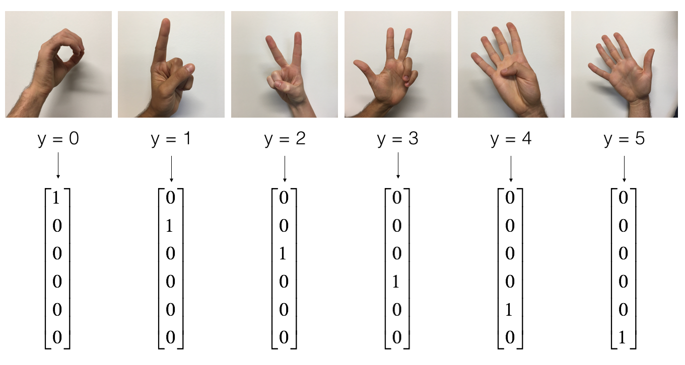
As a reminder, the SIGNS dataset is a collection of 6 signs representing numbers from 0 to 5.
The next cell will show you an example of a labelled image in the dataset. Feel free to change the value of index below and re-run to see different examples.
1 |
|
In Course 2, you had built a fully-connected network for this dataset. But since this is an image dataset, it is more natural to apply a ConvNet to it.
To get started, let's examine the shapes of your data.
1 |
|
1.1 - Create placeholders
TensorFlow requires that you create placeholders for the input data that will be fed into the model when running the session.
Exercise: Implement the function below to create placeholders for the input image X and the output Y. You should not define the number of training examples for the moment. To do so, you could use "None" as the batch size, it will give you the flexibility to choose it later. Hence X should be of dimension [None, n_H0, n_W0, n_C0] and Y should be of dimension [None, n_y]. Hint.
1 |
|
1.2 - Initialize parameters
You will initialize weights/filters \(W1\) and \(W2\) using tf.contrib.layers.xavier_initializer(seed = 0). You don't need to worry about bias variables as you will soon see that TensorFlow functions take care of the bias. Note also that you will only initialize the weights/filters for the conv2d functions. TensorFlow initializes the layers for the fully connected part automatically. We will talk more about that later in this assignment.
Exercise: Implement initialize_parameters(). The dimensions for each group of filters are provided below. Reminder - to initialize a parameter \(W\) of shape [1,2,3,4] in Tensorflow, use:
1 | W = tf.get_variable("W", [1,2,3,4], initializer = ...) |
1 |
|
1 |
|
2 - Forward propagation
In TensorFlow, there are built-in functions that carry out the convolution steps for you.
tf.nn.conv2d(X,W1, strides = [1,s,s,1], padding = 'SAME'): given an input \(X\) and a group of filters \(W1\), this function convolves \(W1\)'s filters on X. The third input ([1,f,f,1]) represents the strides for each dimension of the input (m, n_H_prev, n_W_prev, n_C_prev). You can read the full documentation here
tf.nn.max_pool(A, ksize = [1,f,f,1], strides = [1,s,s,1], padding = 'SAME'): given an input A, this function uses a window of size (f, f) and strides of size (s, s) to carry out max pooling over each window. You can read the full documentation here
tf.nn.relu(Z1): computes the elementwise ReLU of Z1 (which can be any shape). You can read the full documentation here.
tf.contrib.layers.flatten(P): given an input P, this function flattens each example into a 1D vector it while maintaining the batch-size. It returns a flattened tensor with shape [batch_size, k]. You can read the full documentation here.
tf.contrib.layers.fully_connected(F, num_outputs): given a the flattened input F, it returns the output computed using a fully connected layer. You can read the full documentation here.
In the last function above (tf.contrib.layers.fully_connected), the fully connected layer automatically initializes weights in the graph and keeps on training them as you train the model. Hence, you did not need to initialize those weights when initializing the parameters.
Exercise:
Implement the forward_propagation function below to build the following model: CONV2D -> RELU -> MAXPOOL -> CONV2D -> RELU -> MAXPOOL -> FLATTEN -> FULLYCONNECTED. You should use the functions above.
In detail, we will use the following parameters for all the steps: - Conv2D: stride 1, padding is "SAME" - ReLU - Max pool: Use an 8 by 8 filter size and an 8 by 8 stride, padding is "SAME" - Conv2D: stride 1, padding is "SAME" - ReLU - Max pool: Use a 4 by 4 filter size and a 4 by 4 stride, padding is "SAME" - Flatten the previous output. - FULLYCONNECTED (FC) layer: Apply a fully connected layer without an non-linear activation function. Do not call the softmax here. This will result in 6 neurons in the output layer, which then get passed later to a softmax. In TensorFlow, the softmax and cost function are lumped together into a single function, which you'll call in a different function when computing the cost.
1 | # GRADED FUNCTION: forward_propagation |
1 | tf.reset_default_graph() |
3 - Compute cost
Implement the compute cost function below. You might find these two functions helpful:
- tf.nn.softmax_cross_entropy_with_logits(logits = Z3, labels = Y): computes the softmax entropy loss. This function both computes the softmax activation function as well as the resulting loss. You can check the full documentation here.
- tf.reduce_mean: computes the mean of elements across dimensions of a tensor. Use this to sum the losses over all the examples to get the overall cost. You can check the full documentation here.
Exercise: Compute the cost below using the function above.
1 | #GRADED FUNCTION: compute_cost |
1 |
|
4 Model
Finally you will merge the helper functions you implemented above to build a model. You will train it on the SIGNS dataset.
You have implemented random_mini_batches() in the Optimization programming assignment of course 2. Remember that this function returns a list of mini-batches.
Exercise: Complete the function below.
The model below should:
- create placeholders
- initialize parameters
- forward propagate
- compute the cost
- create an optimizer
Finally you will create a session and run a for loop for num_epochs, get the mini-batches, and then for each mini-batch you will optimize the function. Hint for initializing the variables
1 |
|
Run the following cell to train your model for 100 epochs. Check if your cost after epoch 0 and 5 matches our output. If not, stop the cell and go back to your code!
1 | _, _, parameters = model(X_train, Y_train, X_test, Y_test) |
Expected output: although it may not match perfectly, your expected output should be close to ours and your cost value should decrease.
| Cost after epoch 0 = | 1.917929 |
| Cost after epoch 5 = | 1.506757 |
| Train Accuracy = | 0.940741 |
| Test Accuracy = | 0.783333 |
Congratulations! You have finised the assignment and built a model that recognizes SIGN language with almost 80% accuracy on the test set. If you wish, feel free to play around with this dataset further. You can actually improve its accuracy by spending more time tuning the hyperparameters, or using regularization (as this model clearly has a high variance).
Once again, here's a thumbs up for your work!
1 | fname = "images/thumbs_up.jpg" |