本周课程主要讲解了神经网络中的优化的一些方法,要点: - Train/Dev/Test(训练/开发/测试数据集) - 偏差和方差 - 欠拟合和过拟合 - Regularization正则化 - Dropout随机失活 - Normalizing归一化 - 梯度消失和梯度爆炸 - 梯度检查
本周课程将从实际应用的角度介绍深度学习,上周课程已经学会了如何实现一个神经网络,本周将学习,实际应用中如何使神经网络高效工作。本周将学习在实际应用中如何使神经网络高效工作。这些方法包括超参数调整,数据准备,再到如何确保优化算法运行得足够快,以使得学习算法能在合理的时间内完成学习任务。
学习目标
- Recall that different types of initializations lead to different results
- Recognize the importance of initialization in complex neural networks.
- Recognize the difference between train/dev/test sets
- Diagnose the bias and variance issues in your model
- Learn when and how to use regularization methods such as dropout or L2 regularization.
- Understand experimental issues in deep learning such as Vanishing or Exploding gradients and learn how to deal with them
- Use gradient checking to verify the correctness of your backpropagation implementation
课程笔记
Setting up your Machine Learning Application
Train / Dev / Test sets
数据集分为训练集、开发集和测试集。
假设这是你的训练数据,把它画成一个大矩形,那么传统的做法是你可能会从所有数据中,取出一部分用作训练集,然后再留出一部分作为hold-out交叉验证集(hold-out cross validation set)。这个数据集有时也称为开发集,为了简洁,把它称为"dev set"。再接下来从最后取出一部分用作测试集。
整个工作流程:
- 首先不停地用训练集来训练你的算法
- 然后用你的开发集或说hold-out交叉验证集来测试,许多不同的模型里哪一个在开发集上效果最好
- 最后评估最终的训练结果,可以用测试集对结果中最好的模型进行评估,这样以使得评估算法性能时不引入偏差
在上一个时代的机器学习中,通常的分割法是,训练集和测试集分别占整体数据70%和30%。如果你明确地设定了开发集,那比例可能是60/20/20%,也就是测试集占60%,开发集20%,测试集20%,
数年以前这个比例被广泛认为是,机器学习中的最佳方法,如果一共只有100个样本,也许1000个样本,甚至到1万个样本时,这些比例作为最佳选择都是合理的。
但是在这个大数据的时代,趋势可能会变化,可能有多达100万个训练样本,而开发集,和测试集在总体数据中所占的比例就变小了,这是因为,开发集存在的意义是用来,测试不同的算法并确定哪种最好,所以开发集只要足够大到,能够用来在评估两种不同的算法,或是十种不同的算法时快速选出较好的一种,达成这个目标可能不需要多达20%的数据。所以如果有100万个训练样本,可能开发集只要1万个样本就足够了,足够用来评估两种算法中哪一种更好。与开发集相似,测试集的主要功能是,对训练好的分类器的性能,给出可信度较高的评估。同样如果可能有100万个样本,但是只要1万个,就足够评估单个分类器的性能,能够对其性能给出比较准确的估计了。
如果有100万个样本,而只需要1万个用作开发集,1万个用作测试集,那么1万个只是100万个的百分之一,所以比例就是98/1/1%。还有一些应用的样本可能多于100万个,分割比率可能会变成99.5/0.25/0.25%,或者开发集占0.4%,测试集占0.1%。
所以总结起来,当设定机器学习问题时,通常将数据分为训练集,开发集和测试集。如果数据集比较小,也许就可以采用传统的分割比率,但如果数据集大了很多,那也可以使开发集,和测试集远小于总数据20%,甚至远少于10%。
当前的深度学习中还有一个趋势是,有越来越多的人的训练集与测试集的数据分布不匹配。假设构建一个应用,允许用户上传大量图片,目标是找出猫的图片再展示给用户,也许因为用户都是爱猫之人,而训练集可能来自网上下载的猫的图片,而开发集和测试集则包含用户用应用上传的图片,所以,一边是训练集可能有很多从网上爬取的图片,另一边是,开发集和测试集中有许多用户上传的图片,会发现许多网页上的图片都是高分辨率,专业制作过,构图也很漂亮的猫的图片,而用户上传的图则相对比较模糊,分辨率低,用手机在更加随意的情况下拍摄的,所以这可能就造成两种不同的分布,在这种情况下建议的经验法则是,确保开发集和测试集中的数据分布相同。
Make sure that the dev and test sets come from the same distribution.
即使没有测试集也许也是可以的。测试集的目的是给你一个无偏估计,来评价最终所选取的网络的性能。但如果不需要无偏的估计的话,没有测试集也许也没有问题。所以当只有开发集而没有测试集的时候,所做的就是用训练集尝试不同的模型结构,然后用开发集去评估它们,根据结果进一步迭代,并尝试得到一个好的模型,因为模型拟合了开发集中的数据,所以开发集不能给无偏的估计。
Bias / Variance
- Bias,偏差,描述偏离度。
- Variance,方差,描述集中度。

坐标中的⭕和×表示训练集。
左侧是用一条直线来区分样本数据,用逻辑回归可能画出图上的这条直线,这和训练数据的拟合度并不高,这样的分类我们称之为高偏差。或者换一种说法,称为欠拟合。
相对的,右侧的曲线,如果使用一个极为复杂的分类器,或许可以像图上画的这样完美区分训练数据,但看上去也并不是一个非常好的分类算法 这个高方差的分类器,我们也称之为过拟合 。
中间的一条曲线是比较合适的。
训练集的误差,至少可以知道算法是否可以很好的拟合训练集数据,然后总结出是否属于高偏差问题。然后通过观察同一个算法,在开发集上的误差了多少,可以知道这个算法是否有高方差问题。这样就能判断训练集上的算法是否在开发集上同样适用。上述结果都基于贝叶斯误差非常低,并且训练集和开发集都来自与同一个分布。
高偏差高方差的例子如下:
通过观察算法,在训练集和开发集的误差来诊断,它是否有高偏差或者高方差的问题,或许两者都有,或许都没有,基于算法遇到高偏差或高方差问题的不同情况,可以尝试不同的方法来进行改进。
Basic Recipe for Machine Learning
机器学习的基本准则如下图所示:

图中,找到一个新的神经网络结构,这个办法可能有效,也可能无效。把它写在括号里,是因为它是一种需要你亲自尝试的方法,也许最终能使它有效,也许不能。
但在当前这个深度学习和大数据的时代,只要能不断扩大所训练的网络的规模,只要能不断获得更多数据,虽然这两点都不是永远成立的,但如果这两点是可能的,那扩大网络几乎总是能够,减小偏差而不增大方差。只要用恰当的方式正则化的话,而获得更多数据几乎总是能够,减小方差而不增大偏差。
所以归根结底,有了这两步以后,再加上能够选取不同的网络来训练,以及获取更多数据的能力,就有了能够且只单独削减偏差或者能够并且单独削减方差,同时不会过多影响另一个指标的能力。这就是诸多原因中的一个,能够解释为何深度学习在监督学习中如此有用,以及为何在深度学习中,偏差与方差的权衡要不明显得多。这样你就不需小心地平衡两者,而是因为有了更多选择,可以单独削减偏差或单独削减方差,而不会同时增加方差或偏差。而且事实上当有了一个良好地正则化的网络时,训练一个更大的网络几乎从来没有坏处,当训练的神经网络太大时主要的代价只是计算时间。
Regularizing your neural network
Regularization(正则化)
逻辑回归的正则化
\[ \min_{w,b} J(w,b) \] 正则化前: \[ J(w,b) = -\frac{1}{m}\sum_{i=1}^{m}[\mathcal{L}(\hat{y}^{(i)}, y^{(i)})] \]
\(L_2\)正则化后: \[ J(w,b) = -\frac{1}{m}\sum_{i=1}^{m}[\mathcal{L}(\hat{y}^{(i)}, y^{(i)})] + \frac{\lambda}{2m} \parallel w \parallel_2^2 \]
其中,\(\lambda\)是正则化参数。
为什么只对参数w进行正则化呢? 为什么不把b的相关项也加进去呢?实际上可以这样做,但通常会把它省略掉。因为参数\(w\)往往是一个非常高维的参数矢量,尤其是在发生高方差问题的情况下,可能w有非常多的参数。而b只是单个数字,几乎所有的参数都集中在w中,而不是b中。即使你加上了最后这一项,实际上也不会起到太大的作用,因为b只是大量参数中的一个参数,在实践中通常就不费力气去包含它了。
$ L_2$正则化: \[\frac{\lambda}{2m} \parallel w \parallel_2^2 = \frac{\lambda}{2m}\sum_{i=1}^{m}{w_j^2} =\frac{\lambda}{2m} w^Tw\]
$ L_2$正则化是参数矢量w的欧几里得范数的平方。
$ L_1 $正则化: \[\frac{\lambda}{2m} \parallel w \parallel_1 = \frac{\lambda}{2m} \sum_{i=1}^{m}{|w_j|} \]
如果使用$ L_1 \(正则化,最终\)w$会变的稀疏(sparse),也就是包含很多0. 有些人认为这有助于压缩模型,因为有一部分参数是0,只需较少的内存来存储模型。然而在实践中发现,通过L1正则化让模型变得稀疏,带来的收效甚微。所以在压缩模型的目标上,它的作用不大,在训练网络时,L2正则化使用得频繁得多。
注:\(L_1\)范数,表示向量中每个元素绝对值的和:\[ \parallel x \parallel_1 = \sum_{i=1}^{m}{|x_i|} \] \(L_2\)范数,也称为欧几里得距离:\[ \parallel x \parallel_2 = \sqrt{\sum_{i=1}^{m}{x_i^2}} \] L2范数越小,可以使得x的每个元素都很小,接近于0。在回归里面,有人把有它的回归叫“岭回归”(Ridge Regression),有人也叫它权值衰减(Weight Decay)。越小的参数说明模型越简单,越简单的模型则越不容易产生过拟合现象。
神经网络的正则化
正则化前: \[ J(w^{[1]},b^{[1]},\cdots,w^{[l]},b^{[l]}) = -\frac{1}{m}\sum_{i=1}^{m}[\mathcal{L}(\hat{y}^{(i)}, y^{(i)})] \]
正则化后: \[ J(w^{[1]},b^{[1]},\cdots,w^{[l]},b^{[l]}) = -\frac{1}{m}\sum_{i=1}^{m}[\mathcal{L}(\hat{y}^{(i)}, y^{(i)})] + \frac{\lambda}{2m} \sum_{i=1}^{l} \parallel w^{[l]} \parallel_F^2 \]
其中, \[ \parallel w^{[l]} \parallel_F^2 = \sum_{i=1}^{n^{[l-1]}}\sum_{j=1}^{n^{[l]}}(w_{ij}^{[l]})^2 \]
这里矩阵范数的平方定义为,对于i和j,对矩阵中每一个元素的平方求和.如果想为这个求和加上索引,这个求和是i从1到n[l-1],j从1到n[l],因为w是一个n[l-1]列、n[l]行的矩阵,这些是第l-1层和第l层的隐藏单元数量单元数量或这个矩阵的范数,称为矩阵的弗罗贝尼乌斯范数。
\(\lambda\)是正则化参数。
\[ dw^{[l]} = from \,\,backpropagation + \frac{\lambda}{m} w^{[l]}\]
\[ \begin{aligned} w^{[l]} & =w^{[l]} - \alpha dw^{[l]} \\ & = w^{[l]} - \alpha[from \,\,backpropagation + \frac{\lambda}{m} w^{[l]} & = w^{[l]} - \alpha dw^{[l]} \\ & = (1- \frac{\lambda}{m})w^{[l]} - \alpha[from \,\,backpropagation] \end{aligned} \]
从上面的公式中可以看到,\(w^{[l]}\)项前面乘了一个小于1的数,也就是权重会减小,所以这个范数也被称为“权重衰减(weight decay)”。
Why regularization reduces overfitting?
为什么正则化能够防止过拟合呢? 为什么它有助于减少方差问题?
左边是高偏差,右边是高方差,中间的是恰好的情况。
关于这个问题的一个直观理解就是,如果你把正则项λ设置的很大,权重矩阵W就会被设置为非常接近0的值。因此这个直观理解就是:把很多隐藏单元的权重,设置的太接近0了而导致,一些隐藏单元的影响被消除了。如果是这种情况,那么就会使这个大大简化的神经网络变成一个很小的神经网络。事实上,这种情况与逻辑回归单元很像,但很可能是网络的深度更大了,因此这就会使,这个过拟合网络带到更加接近左边高偏差的状态。但是λ存在一个中间值,能够得到一个更加接近中间这个刚刚好的状态。

直觉上认为上图中蓝色被覆盖的部分,这些隐藏单元的影响被完全消除了,其实并不完全正确。实际上网络仍在使用所有的隐藏单元,但每个隐藏单元的影响变得非常小了。但最终得到的这个简单的网络,看起来就像一个不容易过拟合的小型的网络。
现在通过另一个例子直观理解一下,为什么正则化可以帮助防止过拟合,在这个例子中,假设使用的,tanh激活函数。使用\(g(z)\)表示\(tanh(z)\),因此这种情况下,可以发现只要Z的值很小,比如Z只涉及很小范围的参数,tanh曲线中中间的一小部分,那么其实是在使用tanh函数的线性的条件部分。只有Z的值被允许取到更大的值或者像这种小一点的值的时候,激活函数才开始展现出它的非线性的能力。因此直觉就是,如果λ值,即正则化参数被设置的很大的话,那么激活函数的参数实际上会变小,因为代价函数的参数会被不能过大,并且如果W很小那么由于,Z等于W这项再加上b,但如果W非常非常小,那么Z也会非常小。特别是如果Z的值相对都很小时,就在曲线的中间部分范围内取值的话,那么g(z)函数就会接近于线性函数,因此,每一层都几乎是线性的,就像线性回归一样。如果每层都是线性的,那么整个网络就是线性网络。因此即使一个很深的神经网络,如果使用线性激活函数,最终也只能计算线性的函数,因此就不能拟合那些很复杂的决策函数,也不过度拟合那些,数据集的非线性决策平面。
总结一下,如果正则化变得非常大,而参数W很小,那么Z就会相对很小。此时先暂时忽略b的影响,Z会相对变小,即Z只在小范围内取值,那么激活函数如果是tanh的话,这个激活函数就会呈现相对线性,那么整个神经网络就只能计算一些,离线性函数很近的值,也就是相对比较简单的函数,而不能计算,很复杂的非线性函数,因此就不大容易过拟合了。
Dropout Regularization(随机失活正则化(丢弃法))
假设你训练下图所示的神经网络并发现过拟合现象,可以使用随机失活技术来处理它。使用随机失活技术,遍历这个网络的每一层,并且为丢弃(drop)网络中的某个节点置一个概率值(比如50%),即对于网络中的每一层,使这个节点有50%的几率被保留,50%的的几率被丢弃。最后得到的是一个小得多的、被简化了很多的网络。然后再做反向传播训练。
dropout的实现:
有几种方法可以实现随机失活算法,最常用的一种是反向随机失活(inverted dropout) 。
Inverted dropout:反向随机失活的实现:(以3层网络为例)
1 | layer l = 3 |
最后一步的作用是"保证下一层 \(Z^{[4]} = W^{[4]} a^{[3]} + b^{[4]}\) 的期望值不会降低。
测试阶段不使用dropout。
Understanding Dropout
Dropout为什么有效? Can't rely on any one feature,so have to spread out weights.
不同的层,可以设置不同的keep-prop。
如果觉得某一层比其他层更容易发生过拟合,给这一层设置更低的保留率(keep-prop)。这样的缺点是在交叉验证 (网格) 搜索时,会有更多的超参数 (运行会更费时)。另一个选择就是对一些层使用dropout (留存率相同),而另一些不使用。这样的话,就只有一个超参数了。
需要记住dropout是一种正则化技术,目的是防止过拟合。所以,除非算法已经过拟合了,否则是不会考虑使用dropout的。
dropout的另一个缺点是让代价函数J,变得不那么明确。因为每一次迭代,都有一些神经元随机失活,所以检验梯度下降算法表现的时候,会发现很难确定代价函数是否已经定义的足够好 (随着迭代 值不断变小)。通常这个时候可以关闭dropout,把留存率设为1。然后再运行代码并确保代价函数J 是单调递减的,最后再打开dropout并期待使用dropout的时候没有引入别的错误。
Other regularization methods
其他的一些正则化的方法:
- Data augmentation(数据扩增):

- 一只猫,那它水平翻转之后还是一只猫,随机放大图片的一部分,这很可能仍然是一只猫。对于字符识别,可以通过给数字加上随机的旋转和变形。
- Early stoping(早终止法)

- 在某次次迭代附近 ,神经网络表现得最好,然后把神经网络的训练过程停住,并且选取这个(最小)开发集误差所对应的值。
- Early stopiing有个缺点。可以把机器学习过程看作几个不同的步骤,其中之一是:需要一个算法,能够最优化成本函数J。Early stopping的主要缺点就是,它把这两个任务结合了,所以无法分开解决这两个问题。因为提早停止了梯度下降,意味着打断了优化成本函数J的过程。
Setting up your optimization problem
Normalizing inputs
- 均值归一: \[ \mu = \frac{1}{m} \sum_{i=1}^m x^{(i)} \,\,\,\,\,\,\,\,\, x= x - \mu \]
- 方差归一化: \[ \sigma ^ {2} = \frac{1}{m} \sum_{i=1}^m (x^{(i)})^2 \,\,\,\, x= \frac{x}{\sigma ^2} \]

为什么Normalizing有效?

为什么要对输入特征进行归一化呢? 像上图右上方这样的代价函数,如果使用了未归一化的输入特征,代价函数看起来就会像一个压扁了的碗。 如果把这个函数的等值线画出来,就会有一个像这样的扁长的函数。而如果将特征进行归一化后,代价函数通常就会看起来更对称。
如果对左图的那种代价函数使用梯度下降法,那可能必须使用非常小的学习率 。如果等值线更趋近于圆形,那无论从哪儿开始,梯度下降法几乎都能直接朝向最小值而去,可以在梯度下降中采用更长的步长,而无需像左图那样来回摇摆缓慢挪动。
当特征的范围有非常大的不同时,譬如一个特征是1到1000,而另一个是0到1,那就会着实地削弱优化算法的表现了。但只要将它们变换,使均值皆为0,方差皆为1,就能保证所有的特征尺度都相近,这通常也能让帮助学习算法运行得更快。所以如果输入特征的尺度非常不同,比如可能有些特征取值范围是0到1,有些是1到1000,那对输入进行归一化就很重要。而如果输入特征本来尺度就相近,那么这一步就不那么重要。不过因为归一化的步骤几乎从来没有任何害处,所以一般总是进行归一化。
Vanishing / Exploding gradients
当训练神经网络时会遇到一个问题,尤其是当训练层数非常多的神经网络时,这个问题就是梯度消失和梯度爆炸。它的意思是当在训练一个深度神经网络的时候,损失函数的导数,有时会变得非常大,或者非常小甚至是呈指数级减小。

假设:\(g(z)=z,b=0\)
\[ \hat{y} =w^{[l]}w^{[l-1]}w^{[l-2]}\cdots w^{[2]}w^{[1]}x \]
假设:
\[ w^{[l]} = \begin{bmatrix} 1.5 & 0 \\ 0 & 1.5 \\ \end{bmatrix} \]
则 $ = 1.5^{L}x \(,如果L很大,则\)$呈指数级增长。
反之,假设:
\[ w^{[l]} = \begin{bmatrix} 0.5 & 0 \\ 0 & 0.5 \\ \end{bmatrix} \]
则 $ = 0.5^{L}x \(,如果L很大,则\)$会很小。
这就是梯度爆炸或者消失产生的原因。
在这么深的神经网络里,如果激活函数或梯度作为L的函数指数级的增加或减少,这些值会变得非常大或非常小,这会让训练变得非常困难。尤其是如果梯度比L要小指数级别, 梯度下降会很用很小很小步的走,梯度下降会用很长的时间才能有任何学习。
解决梯度爆炸或消失的方法是:谨慎选择初始化权重方法。
Weight Initialization for Deep Networks

如上图的单个的神经元会输入4个特征,从x1到x4,然后用a=g(z)激活,最后得到y。
\[ z = w_1*x_1+w_2*x_2+···+w_n*x_n \,\,\,\,\, b=0\]
为了不让z项太大或者太小,那么n项的数值越大,就会希望\(W_i\)的值越小。因为z是\(w_i*x_i\)的加和。因此,如果加和了很多这样的项,就会希望每一项就尽可能地小。一个合理的做法是,让变量wi等于1/n,这里的n是指输入一个神经元的特征数。
具体做法为:
\[ W^{[l]} = np.random.rand(shape) * np.sqrt(\frac{2}{n^{[l-1]}}) \]
注:这个做法是针对激活函数为\(Rule\)的情况。
虽然这样不能完全解决问题,但它降低了梯度消失和梯度爆炸问题的程度。因为这种做法通过设置权重矩阵W,使得W不会比1大很多,也不会比1小很多。因此梯度不会过快地膨胀或者消失。
其他的激活函数的做法:
- tanh函数(Xavier初始化方法): \[ W^{[l]} = np.random.rand(shape) * np.sqrt(\frac{1}{n^{[l-1]}}) \]
- Rule也可以尝试如下方法: \[ W^{[l]} = np.random.rand(shape) * np.sqrt(\frac{2}{n^{[l]}+ n^{[l-1]}}) \]
Gradient checking
原理是如下公式:
\[ \frac{\partial J}{\partial \theta} = \lim_{\varepsilon \to 0} \frac{J(\theta + \varepsilon) - J(\theta - \varepsilon)}{2 \varepsilon} \]
梯度检查的流程:
- 1.Take \(W^{[1]},b^{[1]},\cdots,W^{[L]},b^{[L]}\) and reshape into a big vector \(\theta\)
- 2.Take \(dW^{[1]},db^{[1]},\cdots,dW^{[L]},db^{[L]}\) and reshape into a big vector \(d\theta\)
- 3.Check: Is \(d\theta\) the gradient of \(J(\theta)\)?
- First compute "gradapprox" using the formula above (1) and a small value of \(\varepsilon\). Here are the Steps to follow:
- \(\theta^{+} = \theta + \varepsilon\)
- \(\theta^{-} = \theta - \varepsilon\)
- \(J^{+} = J(\theta^{+})\)
- \(J^{-} = J(\theta^{-})\)
- \(gradapprox = \frac{J^{+} - J^{-}}{2 \varepsilon}\)
- Then compute the gradient using backward propagation, and store the result in a variable "grad"
- Finally, compute the relative difference between "gradapprox" and the "grad" using the following formula: \[ difference = \frac {\mid\mid grad - gradapprox \mid\mid_2}{\mid\mid grad \mid\mid_2 + \mid\mid gradapprox \mid\mid_2} \] You will need 3 Steps to compute this formula:
- 1'. compute the numerator using np.linalg.norm(...)
- 2'. compute the denominator. You will need to call np.linalg.norm(...) twice.
- 3'. divide them.
- If this difference is small (say less than \(10^{-7}\)), you can be quite confident that you have computed your gradient correctly. Otherwise, there may be a mistake in the gradient computation.
- First compute "gradapprox" using the formula above (1) and a small value of \(\varepsilon\). Here are the Steps to follow:
Gradient Checking Implementation Notes
- Don’t use in training – only to debug
- If algorithm fails grad check, look at components to try to identify bug.
- Remember regularization.
- Doesn’t work with dropout.
- Run at random initialization; perhaps again after some training.
编程练习
Initialization
Welcome to the first assignment of "Improving Deep Neural Networks".
Training your neural network requires specifying an initial value of the weights. A well chosen initialization method will help learning.
If you completed the previous course of this specialization, you probably followed our instructions for weight initialization, and it has worked out so far. But how do you choose the initialization for a new neural network? In this notebook, you will see how different initializations lead to different results.
A well chosen initialization can: - Speed up the convergence of gradient descent - Increase the odds of gradient descent converging to a lower training (and generalization) error
To get started, run the following cell to load the packages and the planar dataset you will try to classify.
1 | import numpy as np |
You would like a classifier to separate the blue dots from the red dots.
1 - Neural Network model
You will use a 3-layer neural network (already implemented for you). Here are the initialization methods you will experiment with:
- Zeros initialization -- setting initialization = "zeros" in the input argument. - Random initialization -- setting initialization = "random" in the input argument. This initializes the weights to large random values.
- He initialization -- setting initialization = "he" in the input argument. This initializes the weights to random values scaled according to a paper by He et al., 2015.
Instructions: Please quickly read over the code below, and run it. In the next part you will implement the three initialization methods that this model() calls.
1 | def model(X, Y, learning_rate = 0.01, num_iterations = 15000, print_cost = True, initialization = "he"): |
2 - Zero initialization
There are two types of parameters to initialize in a neural network: - the weight matrices \((W^{[1]}, W^{[2]}, W^{[3]}, ..., W^{[L-1]}, W^{[L]})\) - the bias vectors \((b^{[1]}, b^{[2]}, b^{[3]}, ..., b^{[L-1]}, b^{[L]})\)
Exercise: Implement the following function to initialize all parameters to zeros. You'll see later that this does not work well since it fails to "break symmetry", but lets try it anyway and see what happens. Use np.zeros((..,..)) with the correct shapes.
1 | # GRADED FUNCTION: initialize_parameters_zeros |
Run the following code to train your model on 15,000 iterations using zeros initialization.
1 | parameters = model(train_X, train_Y, initialization = "zeros") |
1 | Cost after iteration 0: 0.6931471805599453 |
1 | On the train set: |
The performance is really bad, and the cost does not really decrease, and the algorithm performs no better than random guessing. Why? Lets look at the details of the predictions and the decision boundary:
1 | print ("predictions_train = " + str(predictions_train)) |
outputs:
1 | predictions_train = [[0 0 0 0 0 0 0 0 0 0 0 0 0 0 0 0 0 0 0 0 0 0 0 0 0 0 0 0 0 0 0 0 0 0 0 0 0 |
1 | plt.title("Model with Zeros initialization") |
The model is predicting 0 for every example.
In general, initializing all the weights to zero results in the network failing to break symmetry. This means that every neuron in each layer will learn the same thing, and you might as well be training a neural network with \(n^{[l]}=1\) for every layer, and the network is no more powerful than a linear classifier such as logistic regression.
What you should remember: - The weights \(W^{[l]}\) should be initialized randomly to break symmetry. - It is however okay to initialize the biases \(b^{[l]}\) to zeros. Symmetry is still broken so long as \(W^{[l]}\) is initialized randomly.
3 - Random initialization
To break symmetry, lets intialize the weights randomly. Following random initialization, each neuron can then proceed to learn a different function of its inputs. In this exercise, you will see what happens if the weights are intialized randomly, but to very large values.
Exercise: Implement the following function to initialize your weights to large random values (scaled by *10) and your biases to zeros. Use np.random.randn(..,..) * 10 for weights and np.zeros((.., ..)) for biases. We are using a fixed np.random.seed(..) to make sure your "random" weights match ours, so don't worry if running several times your code gives you always the same initial values for the parameters.
1 | # GRADED FUNCTION: initialize_parameters_random |
1 | parameters = initialize_parameters_random([3, 2, 1]) |
1 | W1 = [[ 17.88628473 4.36509851 0.96497468] |
Run the following code to train your model on 15,000 iterations using random initialization.
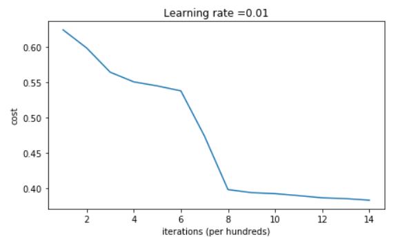
1 | parameters = model(train_X, train_Y, initialization = "random") |
outputs:
1 | Cost after iteration 0: inf |
1 | On the train set: |
If you see "inf" as the cost after the iteration 0, this is because of numerical roundoff; a more numerically sophisticated implementation would fix this. But this isn't worth worrying about for our purposes.
Anyway, it looks like you have broken symmetry, and this gives better results. than before. The model is no longer outputting all 0s.
1 | print (predictions_train) |
*outputs: 1
2
3
4
5
6
7
8
9
10
11
12[[1 0 1 1 0 0 1 1 1 1 1 0 1 0 0 1 0 1 1 0 0 0 1 0 1 1 1 1 1 1 0 1 1 0 0 1 1
1 1 1 1 1 1 0 1 1 1 1 0 1 0 1 1 1 1 0 0 1 1 1 1 0 1 1 0 1 0 1 1 1 1 0 0 0
0 0 1 0 1 0 1 1 1 0 0 1 1 1 1 1 1 0 0 1 1 1 0 1 1 0 1 0 1 1 0 1 1 0 1 0 1
1 0 0 1 0 0 1 1 0 1 1 1 0 1 0 0 1 0 1 1 1 1 1 1 1 0 1 1 0 0 1 1 0 0 0 1 0
1 0 1 0 1 1 1 0 0 1 1 1 1 0 1 1 0 1 0 1 1 0 1 0 1 1 1 1 0 1 1 1 1 0 1 0 1
0 1 1 1 1 0 1 1 0 1 1 0 1 1 0 1 0 1 1 1 0 1 1 1 0 1 0 1 0 0 1 0 1 1 0 1 1
0 1 1 0 1 1 1 0 1 1 1 1 0 1 0 0 1 1 0 1 1 1 0 0 0 1 1 0 1 1 1 1 0 1 1 0 1
1 1 0 0 1 0 0 0 1 0 0 0 1 1 1 1 0 0 0 0 1 1 1 1 0 0 1 1 1 1 1 1 1 0 0 0 1
1 1 1 0]]
[[1 1 1 1 0 1 0 1 1 0 1 1 1 0 0 0 0 1 0 1 0 0 1 0 1 0 1 1 1 1 1 0 0 0 0 1 0
1 1 0 0 1 1 1 1 1 0 1 1 1 0 1 0 1 1 0 1 0 1 0 1 1 1 1 1 1 1 1 1 0 1 0 1 1
1 1 1 0 1 0 0 1 0 0 0 1 1 0 1 1 0 0 0 1 1 0 1 1 0 0]]
1 | plt.title("Model with large random initialization") |
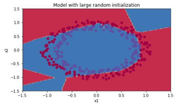
Observations: - The cost starts very high. This is because with large random-valued weights, the last activation (sigmoid) outputs results that are very close to 0 or 1 for some examples, and when it gets that example wrong it incurs a very high loss for that example. Indeed, when \(\log(a^{[3]}) = \log(0)\), the loss goes to infinity. - Poor initialization can lead to vanishing/exploding gradients, which also slows down the optimization algorithm. - If you train this network longer you will see better results, but initializing with overly large random numbers slows down the optimization.
In summary: - Initializing weights to very large random values does not work well. - Hopefully intializing with small random values does better. The important question is: how small should be these random values be? Lets find out in the next part!
4 - He initialization
Finally, try "He Initialization"; this is named for the first author of He et al., 2015. (If you have heard of "Xavier initialization", this is similar except Xavier initialization uses a scaling factor for the weights \(W^{[l]}\) of sqrt(1./layers_dims[l-1]) where He initialization would use sqrt(2./layers_dims[l-1]).)
Exercise: Implement the following function to initialize your parameters with He initialization.
Hint: This function is similar to the previous initialize_parameters_random(...). The only difference is that instead of multiplying np.random.randn(..,..) by 10, you will multiply it by \(\sqrt{\frac{2}{\text{dimension of the previous layer}}}\), which is what He initialization recommends for layers with a ReLU activation.
1 | #GRADED FUNCTION: initialize_parameters_he |
1 | parameters = initialize_parameters_he([2, 4, 1]) |
1 | W1 = [[ 1.78862847 0.43650985] |
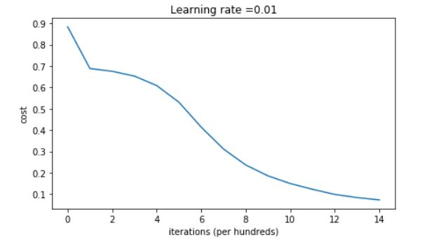
1 | parameters = model(train_X, train_Y, initialization = "he") |
outputs:
1 | Cost after iteration 0: 0.8830537463419761 |
1 | On the train set: |
1 | plt.title("Model with He initialization") |
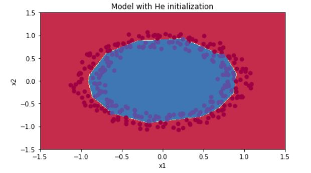
Observations: - The model with He initialization separates the blue and the red dots very well in a small number of iterations.
5 - Conclusions
You have seen three different types of initializations. For the same number of iterations and same hyperparameters the comparison is:
| Model | Train accuracy | Problem/Comment | 3-layer NN with zeros initialization | 50% | fails to break symmetry |
| 3-layer NN with large random initialization | 83% | too large weights |
| 3-layer NN with He initialization | 99% | recommended method |
What you should remember from this notebook: - Different initializations lead to different results - Random initialization is used to break symmetry and make sure different hidden units can learn different things - Don't intialize to values that are too large - He initialization works well for networks with ReLU activations.
Regularization
Welcome to the second assignment of this week. Deep Learning models have so much flexibility and capacity that overfitting can be a serious problem, if the training dataset is not big enough. Sure it does well on the training set, but the learned network doesn't generalize to new examples that it has never seen!
You will learn to: Use regularization in your deep learning models.
Let's first import the packages you are going to use.
1 | import packages |
Problem Statement: You have just been hired as an AI expert by the French Football Corporation. They would like you to recommend positions where France's goal keeper should kick the ball so that the French team's players can then hit it with their head.

They give you the following 2D dataset from France's past 10 games.
1 | train_X, train_Y, test_X, test_Y = load_2D_dataset() |
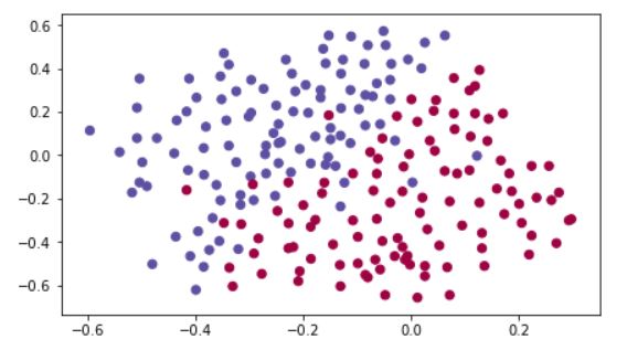
Each dot corresponds to a position on the football field where a football player has hit the ball with his/her head after the French goal keeper has shot the ball from the left side of the football field. - If the dot is blue, it means the French player managed to hit the ball with his/her head - If the dot is red, it means the other team's player hit the ball with their head
Your goal: Use a deep learning model to find the positions on the field where the goalkeeper should kick the ball.
Analysis of the dataset: This dataset is a little noisy, but it looks like a diagonal line separating the upper left half (blue) from the lower right half (red) would work well.
You will first try a non-regularized model. Then you'll learn how to regularize it and decide which model you will choose to solve the French Football Corporation's problem.
1 - Non-regularized model
You will use the following neural network (already implemented for you below). This model can be used: - in regularization mode -- by setting the lambd input to a non-zero value. We use "lambd" instead of "lambda" because "lambda" is a reserved keyword in Python. - in dropout mode -- by setting the keep_prob to a value less than one
You will first try the model without any regularization. Then, you will implement: - L2 regularization -- functions: "compute_cost_with_regularization()" and "backward_propagation_with_regularization()" - Dropout -- functions: "forward_propagation_with_dropout()" and "backward_propagation_with_dropout()"
In each part, you will run this model with the correct inputs so that it calls the functions you've implemented. Take a look at the code below to familiarize yourself with the model.
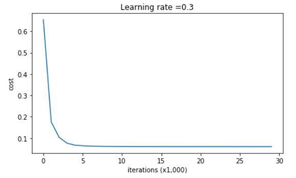
1 | def model(X, Y, learning_rate = 0.3, num_iterations = 30000, print_cost = True, lambd = 0, keep_prob = 1): |
Let's train the model without any regularization, and observe the accuracy on the train/test sets.
1 | parameters = model(train_X, train_Y) |
1 | Cost after iteration 0: 0.6557412523481002 |
1 | On the training set: |
The train accuracy is 94.8% while the test accuracy is 91.5%. This is the baseline model (you will observe the impact of regularization on this model). Run the following code to plot the decision boundary of your model.
1 | plt.title("Model without regularization") |
The non-regularized model is obviously overfitting the training set. It is fitting the noisy points! Lets now look at two techniques to reduce overfitting.
2 - L2 Regularization
The standard way to avoid overfitting is called L2 regularization. It consists of appropriately modifying your cost function, from: \[J = -\frac{1}{m} \sum\limits_{i = 1}^{m} \large{(}\small y^{(i)}\log\left(a^{[L](i)}\right) + (1-y^{(i)})\log\left(1- a^{[L](i)}\right) \large{)} \] To: \[J_{regularized} = \small \underbrace{-\frac{1}{m} \sum\limits_{i = 1}^{m} \large{(}\small y^{(i)}\log\left(a^{[L](i)}\right) + (1-y^{(i)})\log\left(1- a^{[L](i)}\right) \large{)} }_\text{cross-entropy cost} + \underbrace{\frac{1}{m} \frac{\lambda}{2} \sum\limits_l\sum\limits_k\sum\limits_j W_{k,j}^{[l]2} }_\text{L2 regularization cost} \]
Let's modify your cost and observe the consequences.
Exercise: Implement compute_cost_with_regularization() which computes the cost given by formula (2). To calculate \(\sum\limits_k\sum\limits_j W_{k,j}^{[l]2}\) , use : 1
np.sum(np.square(Wl))
1 | # GRADED FUNCTION: compute_cost_with_regularization |
1 | A3, Y_assess, parameters = compute_cost_with_regularization_test_case() |
cost = 1.78648594516
Of course, because you changed the cost, you have to change backward propagation as well! All the gradients have to be computed with respect to this new cost.
Exercise: Implement the changes needed in backward propagation to take into account regularization. The changes only concern dW1, dW2 and dW3. For each, you have to add the regularization term's gradient (\(\frac{d}{dW} ( \frac{1}{2}\frac{\lambda}{m} W^2) = \frac{\lambda}{m} W\)).
1 | # GRADED FUNCTION: backward_propagation_with_regularization |
1 | X_assess, Y_assess, cache = backward_propagation_with_regularization_test_case() |
Output:
1 | dW1 = [[-0.25604646 0.12298827 -0.28297129] |
Let's now run the model with L2 regularization \((\lambda = 0.7)\). The model() function will call: - compute_cost_with_regularization instead of compute_cost - backward_propagation_with_regularization instead of backward_propagation
1 | parameters = model(train_X, train_Y, lambd = 0.7) |
Output:
1 | Cost after iteration 0: 0.6974484493131264 |
1 | On the train set: |
Congrats, the test set accuracy increased to 93%. You have saved the French football team!
You are not overfitting the training data anymore. Let's plot the decision boundary.
1 | plt.title("Model with L2-regularization") |
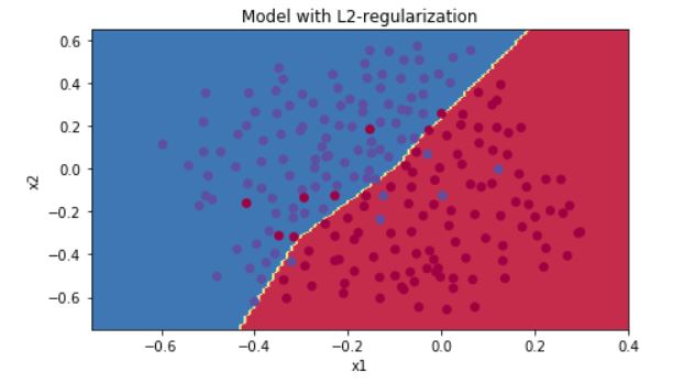
Observations: - The value of \(\lambda\) is a hyperparameter that you can tune using a dev set. - L2 regularization makes your decision boundary smoother. If \(\lambda\) is too large, it is also possible to "oversmooth", resulting in a model with high bias.
What is L2-regularization actually doing?:
L2-regularization relies on the assumption that a model with small weights is simpler than a model with large weights. Thus, by penalizing the square values of the weights in the cost function you drive all the weights to smaller values. It becomes too costly for the cost to have large weights! This leads to a smoother model in which the output changes more slowly as the input changes.
What you should remember -- the implications of L2-regularization on: - The cost computation: - A regularization term is added to the cost - The backpropagation function: - There are extra terms in the gradients with respect to weight matrices - Weights end up smaller ("weight decay"): - Weights are pushed to smaller values.
3 - Dropout
Finally, dropout is a widely used regularization technique that is specific to deep learning. It randomly shuts down some neurons in each iteration. Watch these two videos to see what this means!

At each iteration, you shut down (= set to zero) each neuron of a layer with probability \(1 - keep\_prob\) or keep it with probability \(keep\_prob\) (50% here). The dropped neurons don't contribute to the training in both the forward and backward propagations of the iteration.

\(1^{st}\) layer: we shut down on average 40% of the neurons. \(3^{rd}\) layer: we shut down on average 20% of the neurons.
When you shut some neurons down, you actually modify your model. The idea behind drop-out is that at each iteration, you train a different model that uses only a subset of your neurons. With dropout, your neurons thus become less sensitive to the activation of one other specific neuron, because that other neuron might be shut down at any time.
3.1 - Forward propagation with dropout
Exercise: Implement the forward propagation with dropout. You are using a 3 layer neural network, and will add dropout to the first and second hidden layers. We will not apply dropout to the input layer or output layer.
Instructions: You would like to shut down some neurons in the first and second layers. To do that, you are going to carry out 4 Steps: 1. In lecture, we dicussed creating a variable \(d^{[1]}\) with the same shape as \(a^{[1]}\) using np.random.rand() to randomly get numbers between 0 and 1. Here, you will use a vectorized implementation, so create a random matrix $D^{[1]} = [d^{1} d^{1} ... d^{1}] $ of the same dimension as \(A^{[1]}\). 2. Set each entry of \(D^{[1]}\) to be 0 with probability (1-keep_prob) or 1 with probability (keep_prob), by thresholding values in \(D^{[1]}\) appropriately. Hint: to set all the entries of a matrix X to 0 (if entry is less than 0.5) or 1 (if entry is more than 0.5) you would do: X = (X < 0.5). Note that 0 and 1 are respectively equivalent to False and True. 3. Set \(A^{[1]}\) to \(A^{[1]} * D^{[1]}\). (You are shutting down some neurons). You can think of \(D^{[1]}\) as a mask, so that when it is multiplied with another matrix, it shuts down some of the values. 4. Divide \(A^{[1]}\) by keep_prob. By doing this you are assuring that the result of the cost will still have the same expected value as without drop-out. (This technique is also called inverted dropout.)
1 | #GRADED FUNCTION: forward_propagation_with_dropout |
1 |
|
Output:
A3 = [[ 0.36974721 0.00305176 0.04565099 0.49683389 0.36974721]]
#####3.2 - Backward propagation with dropout
Exercise: Implement the backward propagation with dropout. As before, you are training a 3 layer network. Add dropout to the first and second hidden layers, using the masks \(D^{[1]}\) and \(D^{[2]}\) stored in the cache.
Instruction: Backpropagation with dropout is actually quite easy. You will have to carry out 2 Steps: 1. You had previously shut down some neurons during forward propagation, by applying a mask \(D^{[1]}\) to A1. In backpropagation, you will have to shut down the same neurons, by reapplying the same mask \(D^{[1]}\) to dA1. 2. During forward propagation, you had divided A1 by keep_prob. In backpropagation, you'll therefore have to divide dA1 by keep_prob again (the calculus interpretation is that if \(A^{[1]}\) is scaled by keep_prob, then its derivative \(dA^{[1]}\) is also scaled by the same keep_prob).
1 | # GRADED FUNCTION: backward_propagation_with_dropout |
1 | X_assess, Y_assess, cache = backward_propagation_with_dropout_test_case() |
Output:
1 | dA1 = [[ 0.36544439 0. -0.00188233 0. -0.17408748] |
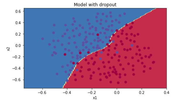
Let's now run the model with dropout (keep_prob = 0.86). It means at every iteration you shut down each neurons of layer 1 and 2 with 14% probability. The function model() will now call: - forward_propagation_with_dropout instead of forward_propagation. - backward_propagation_with_dropout instead of backward_propagation.
1 | parameters = model(train_X, train_Y, keep_prob = 0.86, learning_rate = 0.3) |
Output
1 | Cost after iteration 0: 0.6543912405149825 |
1 | On the train set: |
Dropout works great! The test accuracy has increased again (to 95%)! Your model is not overfitting the training set and does a great job on the test set. The French football team will be forever grateful to you!
Run the code below to plot the decision boundary.
1 |
|
Note: - A common mistake when using dropout is to use it both in training and testing. You should use dropout (randomly eliminate nodes) only in training. - Deep learning frameworks like tensorflow, PaddlePaddle, keras or caffe come with a dropout layer implementation. Don't stress - you will soon learn some of these frameworks.
What you should remember about dropout: - Dropout is a regularization technique. - You only use dropout during training. Don't use dropout (randomly eliminate nodes) during test time. - Apply dropout both during forward and backward propagation. - During training time, divide each dropout layer by keep_prob to keep the same expected value for the activations. For example, if keep_prob is 0.5, then we will on average shut down half the nodes, so the output will be scaled by 0.5 since only the remaining half are contributing to the solution. Dividing by 0.5 is equivalent to multiplying by 2. Hence, the output now has the same expected value. You can check that this works even when keep_prob is other values than 0.5.
4 - Conclusions
Here are the results of our three models:
| model | train accuracy | test accuracy | 3-layer NN without regularization | 95% | 91.5% |
| 3-layer NN with L2-regularization | 94% | 93% |
| 3-layer NN with dropout | 93% | 95% |
Note that regularization hurts training set performance! This is because it limits the ability of the network to overfit to the training set. But since it ultimately gives better test accuracy, it is helping your system.
Congratulations for finishing this assignment! And also for revolutionizing French football. :-)
What we want you to remember from this notebook: - Regularization will help you reduce overfitting. - Regularization will drive your weights to lower values. - L2 regularization and Dropout are two very effective regularization techniques.
Gradient Checking
Welcome to the final assignment for this week! In this assignment you will learn to implement and use gradient checking.
You are part of a team working to make mobile payments available globally, and are asked to build a deep learning model to detect fraud--whenever someone makes a payment, you want to see if the payment might be fraudulent, such as if the user's account has been taken over by a hacker.
But backpropagation is quite challenging to implement, and sometimes has bugs. Because this is a mission-critical application, your company's CEO wants to be really certain that your implementation of backpropagation is correct. Your CEO says, "Give me a proof that your backpropagation is actually working!" To give this reassurance, you are going to use "gradient checking".
Let's do it!
1 | import numpy as np |
1) How does gradient checking work?
Backpropagation computes the gradients \(\frac{\partial J}{\partial \theta}\), where \(\theta\) denotes the parameters of the model. \(J\) is computed using forward propagation and your loss function.
Because forward propagation is relatively easy to implement, you're confident you got that right, and so you're almost 100% sure that you're computing the cost \(J\) correctly. Thus, you can use your code for computing \(J\) to verify the code for computing \(\frac{\partial J}{\partial \theta}\).
Let's look back at the definition of a derivative (or gradient): \[ \frac{\partial J}{\partial \theta} = \lim_{\varepsilon \to 0} \frac{J(\theta + \varepsilon) - J(\theta - \varepsilon)}{2 \varepsilon} \]
If you're not familiar with the "\(\displaystyle \lim_{\varepsilon \to 0}\)" notation, it's just a way of saying "when \(\varepsilon\) is really really small."
We know the following:
- \(\frac{\partial J}{\partial \theta}\) is what you want to make sure you're computing correctly.
- You can compute \(J(\theta + \varepsilon)\) and \(J(\theta - \varepsilon)\) (in the case that \(\theta\) is a real number), since you're confident your implementation for \(J\) is correct.
Lets use equation (1) and a small value for \(\varepsilon\) to convince your CEO that your code for computing \(\frac{\partial J}{\partial \theta}\) is correct!
2) 1-dimensional gradient checking
Consider a 1D linear function \(J(\theta) = \theta x\). The model contains only a single real-valued parameter \(\theta\), and takes \(x\) as input.
You will implement code to compute \(J(.)\) and its derivative \(\frac{\partial J}{\partial \theta}\). You will then use gradient checking to make sure your derivative computation for \(J\) is correct.

The diagram above shows the key computation steps: First start with \(x\), then evaluate the function \(J(x)\) ("forward propagation"). Then compute the derivative \(\frac{\partial J}{\partial \theta}\) ("backward propagation").
Exercise: implement "forward propagation" and "backward propagation" for this simple function. I.e., compute both \(J(.)\) ("forward propagation") and its derivative with respect to \(\theta\) ("backward propagation"), in two separate functions.
1 | # GRADED FUNCTION: forward_propagation |
Exercise: Now, implement the backward propagation step (derivative computation) of Figure 1. That is, compute the derivative of \(J(\theta) = \theta x\) with respect to \(\theta\). To save you from doing the calculus, you should get \(dtheta = \frac { \partial J }{ \partial \theta} = x\).
1 | # GRADED FUNCTION: backward_propagation |
Exercise: To show that the backward_propagation() function is correctly computing the gradient \(\frac{\partial J}{\partial \theta}\), let's implement gradient checking.
Instructions: - First compute "gradapprox" using the formula above (1) and a small value of \(\varepsilon\). Here are the Steps to follow: 1. \(\theta^{+} = \theta + \varepsilon\) 2. \(\theta^{-} = \theta - \varepsilon\) 3. \(J^{+} = J(\theta^{+})\) 4. \(J^{-} = J(\theta^{-})\) 5. \(gradapprox = \frac{J^{+} - J^{-}}{2 \varepsilon}\) - Then compute the gradient using backward propagation, and store the result in a variable "grad" - Finally, compute the relative difference between "gradapprox" and the "grad" using the following formula: \[ difference = \frac {\mid\mid grad - gradapprox \mid\mid_2}{\mid\mid grad \mid\mid_2 + \mid\mid gradapprox \mid\mid_2} \] You will need 3 Steps to compute this formula: - 1'. compute the numerator using np.linalg.norm(...) - 2'. compute the denominator. You will need to call np.linalg.norm(...) twice. - 3'. divide them. - If this difference is small (say less than \(10^{-7}\)), you can be quite confident that you have computed your gradient correctly. Otherwise, there may be a mistake in the gradient computation.
1 | #GRADED FUNCTION: gradient_check |
1 | x, theta = 2, 4 |
Expected Output:
The gradient is correct! difference 2.9193358103083e-10
Congrats, the difference is smaller than the \(10^{-7}\) threshold. So you can have high confidence that you've correctly computed the gradient in backward_propagation().
Now, in the more general case, your cost function \(J\) has more than a single 1D input. When you are training a neural network, \(\theta\) actually consists of multiple matrices \(W^{[l]}\) and biases \(b^{[l]}\)! It is important to know how to do a gradient check with higher-dimensional inputs. Let's do it!
3) N-dimensional gradient checking
The following figure describes the forward and backward propagation of your fraud detection model.

Let's look at your implementations for forward propagation and backward propagation.
1 | def forward_propagation_n(X, Y, parameters): |
Now, run backward propagation.
1 | def backward_propagation_n(X, Y, cache): |
You obtained some results on the fraud detection test set but you are not 100% sure of your model. Nobody's perfect! Let's implement gradient checking to verify if your gradients are correct.
How does gradient checking work?.
As in 1) and 2), you want to compare "gradapprox" to the gradient computed by backpropagation. The formula is still:
\[ \frac{\partial J}{\partial \theta} = \lim_{\varepsilon \to 0} \frac{J(\theta + \varepsilon) - J(\theta - \varepsilon)}{2 \varepsilon} \]
However, \(\theta\) is not a scalar anymore. It is a dictionary called "parameters". We implemented a function "dictionary_to_vector()" for you. It converts the "parameters" dictionary into a vector called "values", obtained by reshaping all parameters (W1, b1, W2, b2, W3, b3) into vectors and concatenating them.
The inverse function is "vector_to_dictionary" which outputs back the "parameters" dictionary.
 and vector_to_dictionary().You will need these functions in gradient_check_n()")
We have also converted the "gradients" dictionary into a vector "grad" using gradients_to_vector(). You don't need to worry about that.
Exercise: Implement gradient_check_n().
Instructions: Here is pseudo-code that will help you implement the gradient check.
For each i in num_parameters: - To compute J_plus[i]: 1. Set \(\theta^{+}\) to np.copy(parameters_values) 2. Set \(\theta^{+}_i\) to \(\theta^{+}_i + \varepsilon\) 3. Calculate \(J^{+}_i\) using to forward_propagation_n(x, y, vector_to_dictionary(\(\theta^{+}\) )).
- To compute J_minus[i]: do the same thing with \(\theta^{-}\) - Compute \(gradapprox[i] = \frac{J^{+}_i - J^{-}_i}{2 \varepsilon}\)
Thus, you get a vector gradapprox, where gradapprox[i] is an approximation of the gradient with respect to parameter_values[i]. You can now compare this gradapprox vector to the gradients vector from backpropagation. Just like for the 1D case (Steps 1', 2', 3'), compute: \[ difference = \frac {\| grad - gradapprox \|_2}{\| grad \|_2 + \| gradapprox \|_2 } \]
1 | # GRADED FUNCTION: gradient_check_n |
1 | X, Y, parameters = gradient_check_n_test_case() |
Expected output:
There is a mistake in the backward propagation! difference = 0.285093156781
It seems that there were errors in the backward_propagation_n code we gave you! Good that you've implemented the gradient check. Go back to backward_propagation and try to find/correct the errors (Hint: check dW2 and db1). Rerun the gradient check when you think you've fixed it. Remember you'll need to re-execute the cell defining backward_propagation_n() if you modify the code.
Can you get gradient check to declare your derivative computation correct? Even though this part of the assignment isn't graded, we strongly urge you to try to find the bug and re-run gradient check until you're convinced backprop is now correctly implemented.
Note - Gradient Checking is slow! Approximating the gradient with \(\frac{\partial J}{\partial \theta} \approx \frac{J(\theta + \varepsilon) - J(\theta - \varepsilon)}{2 \varepsilon}\) is computationally costly. For this reason, we don't run gradient checking at every iteration during training. Just a few times to check if the gradient is correct. - Gradient Checking, at least as we've presented it, doesn't work with dropout. You would usually run the gradient check algorithm without dropout to make sure your backprop is correct, then add dropout.
Congrats, you can be confident that your deep learning model for fraud detection is working correctly! You can even use this to convince your CEO. :)
What you should remember from this notebook: - Gradient checking verifies closeness between the gradients from backpropagation and the numerical approximation of the gradient (computed using forward propagation). - Gradient checking is slow, so we don't run it in every iteration of training. You would usually run it only to make sure your code is correct, then turn it off and use backprop for the actual learning process.